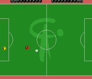
Fig 1: A snapshot taken during
a game on the SoccerServer
The main objective of this project is to develop a client for the standard Noda SoccerServer environment using the layered machine learning approach. The skills incorporated would be :
SoccerServer
The SoccerServer is a standard testbed for new theories on Machine Learning
and Multi-Agent Systems. It was originally developed by Itsuki Noda and
is used every year for the simulated version of the RoboSoccer world cup.
The SoccerServer is a complex and realistic domain. It embraces as many
real-world complexities as possible - all motions are randomized, no communication
is completely safe, no input data is totally reliable and the stamina of
each agent is limited.
Several clients can connect together to the SoccerServer via UDP sockets.
The SoccerServer is responsible for conducting the game according to the
rules. It periodically sends out visual and audio data to each client according
to what lies in its field of view/vision.
Fig 1: A snapshot taken during
a game on the SoccerServer
For example in the position shown above, consecutive packets received by
the client are:
(see 144 ((goal
r) 95.6 -11) ((flag c b) 49.9 24) ((flag r t) 104.6 -30) ((flag r b) 98.5
8) ((flag p r t) 83.9 -26) ((flag p r c) 79 -12) ((flag p r b) 79.8 2)
((ball) 33.1 -2 0 0) ((player pakistan 1) 20.1 -10 0.402 0.4) ((line r)
95.6 83))
(see 145 ((goal
r) 95.6 -9) ((flag c b) 49.9 26) ((flag r t) 104.6 -28) ((flag r b) 98.5
10) ((flag p r t) 83.9 -24) ((flag p r c) 79 -10) ((flag p r b) 79.8 4)
((ball) 33.1 0 0 -0) ((player pakistan 1) 20.1 -7 0.402 0.2) ((line r)
95.6 85))
(see 147 ((goal
r) 94.6 -9) ((flag c b) 49.4 27) ((flag r t) 103.5 -28) ((flag r b) 97.5
10) (flag p r t) 83.1 -24) ((flag p r c) 78.3 -10) ((flag p r b) 79 4)
((ball) 33.1 0) ((player pakistan 1) 22.2 -6 -0 0.1) ((line r) 94.6 85))
Each packet
gives the relative distance and direction of the other objects within the
field of view.
Note that
the packet at time cycle 146 is missing. This is because of the unreliability
of the communication and complicates matters further. During extended runs,
it was observed that only about 60% of packets reach the destination.
Each client acts as the brain of one player, and it send commands to the
server. These are processed by the server which thus acts as a physical
world for the clients.
Our task is thus to model the brain
of the agent, which links sensory inputs to actuation.
Past Work
Robot soccer
was initiated in the mid 90's as a competitive sport.
The first
robot to play soccer, Dynamite, was developed in 1994. And soccer robots
have not looked back since then.
The recent
contributions to this field have come from the Carnegie Mellon robot soccer
team CMUnited that has rocked the recent robocups with its dazzling performance.
We concentrate on
the approach in Peter Stone's thesis work on Layered Learning in Multi-Agent
Systems. His work is based on a practical approach to learning in the presence
of noise. He also describes techniques for agent coordination and effective
teamwork.
Sreangshu Acharya
has developed the lower layers of our system (shooting and interception)
and we will use his modules in our project.
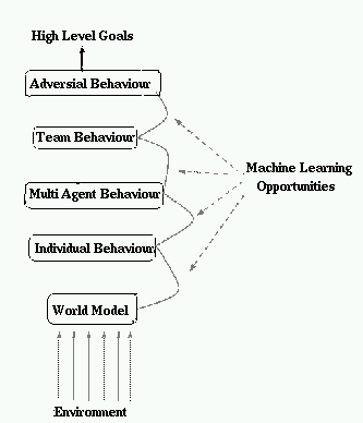
GeneralOverview
As we view it, our project has the following logical course:
Before we proceed, an introduction to radial basis function networks is essential. After that, we would continue to describe the stages above.
Radial Basis Function Networks
Radial basis function networks (RBFNs) are a special class of Artificial Neural Networks (ANNs). They can be used to model any function from one space to the other. They are thus versatile function generalizers.
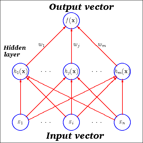
Topology of a single output radial basis function network : x is the input vector, w's are the weights and h()'s are the radial basis activation functions
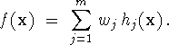
They contain
a single hidden layer of neurons that are completely linked to the input
and output layers. The transfer function in the hidden layer is a non-linear
function with radial symmetry, i.e., the value depends only on the distance
of the point from the centre of that unit.
Here the Gaussian
activation function is used (which means distances are Euclidean), with
the parameters r (the radius or sigma) and c (centre taken from the input
space) defined separately at each RBF unit.
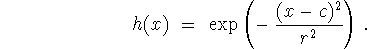
Generally the activation function is bell-shaped with a maximum at the centre and almost zero far away. This allows incremental learning, in which a unit of the network can be modified without affecting the overall behaviour. Moreover, the basic advantage over ANNs is that RBFNs have tractable physical interpretations. They can be interpreted as a series of local receptors, because each unit handles the data points sufficiently close to it.
For RBFNs to be used as function approximators, there must be a regression method that chooses the parameters (centres, sigmas and weights) in such a way as to minimize the error at the training set points while avoiding overfitting. Such a method should lead to good function generalization over the whole input space. The regression method used here involves hard clustering for finding the centres, heuristics to find the sigma and linear regression to find the weights. For details on these algorithms, click here.
Machine learning
Machine learning
is the most versatile tool to impart domain knowledge to an AI agent. The
idea is that the rules of the world are not hand coded by the programmer
but are found out by the agent through exploration of the its environment.
The learning
process is classified in several ways.
Supervised
and unsupervised learning : In supervised learning a target function
is given through a set of instances (mapping values at some points) and
the problem reduces to a regression problem (assuming a continuous function).
With unsupervised learning, no target function is available, so the problem
is to discover the functional relationship among the data.
Reinforcement
learning is a partially supervised learning technique - no correct answer
is known at the outset, but the system receives rewards or punishments
that implicitly contain information on the target function.
Off-line and on-line learning : In off-line learning, the system is completely focussed on the learning activity and the set of samples is given completely at the beginning. But in on-line learning, there is no strict separation between the learning phase and the task-execution phase. Learning is done step by step as fresh data becomes available.
Layered learning
The problem
with machine learning as such is that in a complex and noisy system, where
no simple relations connect the input to the output, it is not possible
to directly learn the input-output mapping. Consider for example the case
of robotic soccer. Theoretically, we can get over the problem in one step
- all the coordinates of all the objects and their face directions
(where applicable) define the state of the game completely and can be used
as the input space (this will have about 68 dimensions, 3 for each of the
22 players and 2 for the ball). Learning can be done so that we get the
optimal action to be taken (kick, dash, turn etc.) and the relevant parameters
for that action at once. But a look at the dimensionality of this approach
shows that the learning time involved is prohibitive. Further, any small
change in one parameter, and the whole training must be repeated.
To conquer
this curse of dimensionality, we use Peter Stone's layered learning approach
. The idea here is that the task is subdivided into layers and machine
learning techniques are applied separately at each layer. The agent first
learns the basic skills such as kicking and intercepting, then uses these
to dribble, then proceeds to team behaviour and so on.
Reinforcement learning
The basic problem
with normal supervised learning is that in some complicated real-world
situations (say, a flight simulator) it is difficult to give the optimum
output for data points. In such cases, reinforcement learning (RL) provides
a powerful learning framework.
In RL, the
system is just given a goal to achieve. In theory, this can be as basic
an objective as possible (e.g the goal for the flight simulator agent may
be to make a safe landing). The system interacts with the environment and
tries to achieve the goal by trial and error interactions with the environment.
Favourable actions result in a reward from the environment while others
may be punished.
This illustrates
the basic idea, but there are several finer points to note.
Exploration
and exploitation : As an agent learns by interacting with its environment,
it has two broad courses of action - it may decide to explore the environment
further by choosing suboptimal actions to expand its knowledge (exploration),
or, it may decide to choose the optimal action suggested by the current
knowledge of the agent (exploitation). Exploration is necessary to discover
optimal solutions in an unknown environment, but when in excess, it leads
to wastage of time and energy. Thus a balance must be reached for which
several exploration decay schemes have been proposed.
We now return to the actual work done by us.
DEVELOPMENT OF A BASIC CLIENT MODULE
For this, we
built on standard Java code available with SoccerServer 4.21.
A major hurdle
was making sense of the loads of data received several times a second from
the server. This must be parsed and the internal data structures must be
updated for use by the agent's brain. This component is called the agent's
memory and incorporates a basic world model.
A client's world model
Since all coordinates
given in a server packet are relative, the first step must be to
obtain self coordinates on the field. Because of the noisy and unreliable
communication and the randomness of the system, the agent cannot simply
process all the commands it sends to the server and calculate the expected
results from these. Instead, self coordinates must themselves be obtained
by observing how the fixed objects on the field (lines, goals and flags)
are seen from that location (distance and relative angle).
The server
packet is parsed and when two fixed objects are found, they are used to
identify the location and the facing direction of the self client. This
process is called triangulation.
Once the self
coordinates and velocities are obtained, the other parts of the packet
begin to make sense and they are stored as such in relative coordinates
to avoid excessive computations. Here we assume that all directly observed
data is accurate, as this suffices for our purposes. In other words, the
confidence value of directly observed data is assumed to be 1.
The objects
that are not within the field of view are not included in the server packet.
To maintain a reasonable world model, these are extrapolated to a new location
by considering a decaying velocity (velocity is obtained below). The confidence
value is decayed each time such an extrapolation is performed, and once
it falls below a certain threshold, the information about that object is
deemed absent.
Ghost objects : These are objects which are supposed to be in the field of view according to the memory model but are not actually observed. These constitute imaginary objects and are disregarded by setting their confidence value to 0.
Obtaining an object's velocity
Velocity is obtained in a simple fashion by comparing two consecutive observations when self triangulation was performed and thus coordinates of all field objects were obtained. A problem faced here is that the several factors such as noise and randomness lead to very misleading velocity calculations. This is to be expected because an object moving in a straight line actually moves in a zig zag random manner along this general direction. It is essential to obtain some sort of an average to guide the client in actions such as interception.
For example,
suppose a client is watching a ball that is kicked by an opponent player
at right angles to its viewing direction. The following data were calculated
from subsequent packets received from the server :
| Time step when packet was received | Xball (calculated) | Yball (calculated) | Vx (direct) | Vy (direct) | Vx (model) | Vy (model) |
| 24 | 1.4533 | -1.2060 | 1.0108 | -0.5469 | 0.0684 | 0.0198 |
| 25 | 1.4049 | 0.0868 | -0.0484 | 1.2928 | 0.051731553 | 0.2017 |
| 27 (opponent kick) | 0.6727 | -0.9077 | -0.3661 | -0.9945 | -0.0411 | 0.0464 |
| 28 | 2.1724 | 0.4964 | 1.4997 | 1.4041 | (kick detected) 1.0374 | 0.9969 |
| 30 | 5.2577 | -0.3359 | 1.5427 | -0.4162 | 1.3742 | 0.05482014 |
| 32 | 6.7696 | -0.6967 | 0.7560 | -0.1804 | 1.1269 | -0.0392 |
| 33 | 8.4820 | -0.6918 | 1.7124 | -0.0049 | 1.2245 | -0.0319 |
| 35 | 10.4873 | -1.0720 | 1.0027 | -0.1901 | 1.1690 | -0.0714 |
It is clear from the table that the instantaneous velocity provides a poor estimate.
Vnew=lambda * Vold + (1-lambda) * (ds/dt)new
where lambda (=1/3 in our case) represents a smoothing factor. Higher the value of lambda, more is the weightage given to the previous values in the new velocity.
This smoothes the velocity function to an extent, but problems persist. Specifically, the client is unable to detect the kick and mixes up the pre-kick and post-kick periods which does not give good enough results.
In essence,
the averaging must be done over a larger range of time.
For this,
the client calculates the instantaneous velocity estimate and checks if
its vector difference from the earlier velocity is greater than a threshold
magnitude Vth. If it is, then the client recognizes a transition
for the ball and records that location. Subsequently, all velocity estimations
are derived by an average starting from that transition instant. In effect,
this separates the post-kick period from the pre-kick period, while at
the same time maintaining a reliable average of the velocity when transitions
do not occur. The velocity remains stable, but varies sharply at transition
instants.
Experimentally,
it was found that any single threshold Vth does not separate
kicks from spurious noise.
So a dynamic threshold was used with the following two
variables :
The interception module results show the advantage of this velocity model of the ball.
The coach client
Controlling
the simulations on the SoccerServer is difficult without a specialized
tool. For this, the Server provides the facility of a coach client.
Its mode of communication with the server is similar, but it receives the
accurate position of each object on the field at each time cycle. In this
sense, it is like an overhead camera placed over the field of play.
We developed
a coach client that basically sets the players and the ball to a practice
position, performs a simulation and observes the results. It includes a
trigger condition that decides when the simulation is to end and the reinforcements
are to be evaluated. The coach client makes generation of the training
set easy through actual simulations on the SoccerServer. This is described
further in the section on dribbling learning.
The shooting module
Here we used
the code developed by Sreangshu Acharya as our basic framework. But the
whole training process had to be done from the beginning as his work was
not done with the actual simulator parameters.
First a set
of training positions is generated with the shooter in possession of the
ball and at most three opponents, of which one may be the goalie. Thus
the input vector has 8 components.
These were
learnt (without simulations) to generate the optimal shooting angle for
each and thus complete the training set. Each position is given two outputs,
the optimal shooting angle and the probability of scoring a goal.
This mapping
from the 8 dimension input space to the 2 dimension output space was then
modeled by a RBFN. For this regression process, hard clustering was used
to determine the centres and the sigmas were determined empirically. The
weights can then be found using simple linear regression.
The training
set generalization was acceptable and the output on inputs previously unknown
to the network is quite accurate.
To view some
sample outputs, click here.
The interceptor module
The interception
process is quite similar. The input vector now contains five components
as shown below.
The earlier
methods developed using RBF's involved either involved evaluating a separately
trained RBFN for each interception velocity and the time cycle for interception,
or, given a fixed interception velocity, use a trained RBFN to find
the best interception step. We did not get good results with either of
these as they either cannot be implemented in real time or did not generalize
well over the input space.
So we decided
to use simple geometry for this.
The client
uses its velocity model of the ball to calculate the earliest instant of
time where it can intercept the ball. This is done by actually calculating
the location of the ball at each instant using the decay parameters of
the SoccerServer. For this, it considers only the most probable position of the ball rather than considering its fuzzy distribution over
neighbouring points also. The assumption may not be completely correct
but gives good results. If the client has to plan to move to a point where
it expects to find the ball, this position will at most be only slightly
distant from the position calculated using the most probable position model.
This optimal
interception position calculated is treated as a planned position for interception.
The client tries to move straight to this point. In subsequent cycle, unless
the planned position changes drastically (which does not generally happen
in our stable velocity model) , the client continues to dash to this position.
Thus it saves cycles by not turning unnecessarily.
To view some sample outputs, click here.
STRATEGIC POSITIONING OF PASSIVE AGENTS
Good team play
is not possible unless the clients play with good "soccer sense". When
a client does not have the ball (i.e., when the agent is passive), he should
use his time and stamina effectively to position itself in such a way that
facilitates further play.
For this purpose
we use Strategic Positioning by Attraction and Repulsion (SPAR) developed
by the CMUnited team. The idea here is that a passive agent should move
close to the opponent goal while keeping away from opponents (to tackle
defence), teammates (to play a "spread out" game) and boundaries (to not
get away from the centre too much). As a special case, the far boundary
of the field is considered to be in the same line as the last defender
on the opposing team (this is done to avoid offsides). The method used
is to consider each of these as charges and imagine a potential field around
these (here we try to maximize this potential value). The potential
function used by us is :
V(p,s)= a * (sum of distance of p to other players) -
b * exp(-dist(p, each player)2/sigma1)
- c * exp(-distance from boundaries/sigma2)
- d * (distance to opponent goal)2
As mentioned
above, the second term treats the opponent goal boundary at the offside
location determined from the defender locations.
In this formula,
a, b, c and d are constants representing relative weights and were determined
experimentally. Note that two terms are used to keep the client away from
other players - the first linear term gives a general tendency to move
as far away as possible while the second Gaussian term further discourages
the agent from coming too close to any player on the field.
Also, the
sigma2 value is low to provide a steep fall at the boundaries.
Note that in
an actual game, most of the objects are not in the client's field of view.
They are obtained from the memory model.
To view plots
of how this potential function spreads over the field, click
here.
Ideally, each passive client should find the maximum potential and move towards it. But a global search is neither possible in real-time, nor are we interested in the global maximum because by the time the client gets there, it may be too late. On the other hand, choosing the locally optimum solution (i.e. moving down the potential hill at every point) would frequently end up in local maxima that don't give optimum results.
Thus we use
an intermediate approach. The agent looks for the best position in an imaginary
grid around it, where the size of the grid to search represents the maximum
distance that the agent can move without taking too much time. The grid
location that gives the maximum potential is considered to be the most
favourable location for the agent.
However a
naive application of this means that the client is just stuck up turning
at its own location. This is because the optimum location may switch rapidly
between neighbouring points in a dynamic game. If the agent tries to move
to the best point at each time cycle, it must first turn in the right direction
before dashing, but before it is ready to dash, the target location shifts
again.
To counter
this, we develop the idea of a plan. The agent applies the above grid algorithm,
finds the optimal location and generates a "plan" to move there. Subsequently,
if the optimal points are either within a certain distance of the old point
or are within a small cone, they are not used to changed the plan. This
means that the agent can use time cycles for actual dashing rather than
just turning to no use.
To view some
of the results obtained, click here.
LEARNING TO DRIBBLE
We define dribbling
to be the actions of a player with the ball that allow it to keep possession
while moving it "usefully". The power of reinforcement learning lies in
the fact that the utility of an action can be described in very basic terms
such as the distance advanced towards goal or the time taken to get to
the ball again. All the complications are handled by the learning procedure.
The positions
considered here consist of two players per team, with the agent doing the
learning within kickable distance of the ball. The passive teammate is
endowed with strategic positioning through SPAR (described earlier). The
opponents have already learnt the interception skill in a lower layer.
This demonstrates the power of layered learning - a learned behaviour is
used to provide further knowledge in subsequent learning runs.
We use RBFNs
for learning because the domain is continuous and complex. The input vector
to the network consists of 8 components, two per player, with the distances
given in inverse polar form and the other coordinate given as a relative
angle. The expected output is the optimal dribbling angle and velocity
of the kick. The steps to be followed are described below.
Generation of training set positions
For good generalization results, the training set should reflect the positions that are expected to arise in a real game - more frequent positions should get more representation. The weights are hand-coded and some heuristics are applied to remove the useless positions (e.g. if the opponents are very far back, they can be treated as absent). Finally, about 540 positions have been obtained that span the expected parts of the input space. This number may be increased if the generalization observed is inadequate.
Obtaining the optimal output for a training position
This is the
main part of the learning procedure.
We use actual
simulations to find the optimal output for each input position. Though
this takes more time, the training is more exact as it is done in the noisy
and random environment where it will ultimately be used.
The search
for the optimal values of the kicking angle and velocity is done in stages.
Instead of considering a continuous variation in these values, the search
evaluates these at certain values only. Here heuristics are used so that
the density of angle values considered is higher in the goalward direction
and very low in the backward direction.
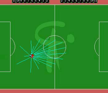
Fig : The red player is learning dribbling and shooting
towards right.
The angle and velocity combinations are schematically
sketched.
Note the significantly higher concentration towards the
opponent goal.
Now several simulations are conducted from this position. For this the coach client is invaluable - it moves the objects to positions prespecified in a file and waits till a trigger condition is reached. This trigger condition may be caused by the ball coming within kickable distance of one of the four players, going into the goal or going out of bounds or a final case when none of these happens for a specified length of time from the start. When any of these is satisfied, the coach evaluates a reinforcement function based on the final position of the players and the type of trigger. This reinforcement is passed on to the learning client over the network through an audio message.
Suppose that when the trigger condition is reached, the following values are obtained (as the coach client gets the global coordinates at each cycle, it can easily obtain these values:
Decrease in distance from opponent goal = d (metres)
Time taken before the trigger condition is reached =
T (time cycles)
Sum of distances of active agent from two opponent players
= D (metres)
Distances from individual opponents = d1, d2 (metres)
Minimum relative angle between with teammate and an opponent
player = theta (in radians)
If the passive teammate is closer than the defender forming the angle theta, theta is given a high value to show that the defender is not in an intercepting position.
The values D and theta are used to heuristically estimate the utility of the position reached in the end. To see what they mean, click here.
The reinforcement
function then is : (this part has not been completed, so the form of the
reinforcement function and the constants will change a bit with experimentation)
| Type of trigger condition | Reinforcement provided (R) |
| Ball returns to self | + 9
+ 5 * P(goal/shoot) (to account for goal scoring possibilty from new position) + 15 * d / (40 + T) (to encourage agent to decrease distance to goal quickly) + D / 20 (to encourage agent to keep away from defence in general) - 5 * exp(-d12/20) (to discourage agent from coming too close to any one - 5 * exp(-d22/20) defender) + 2 * theta (to improve passing to teammate) |
| Ball into opponent goal | +30 |
| Ball into self goal | -25 |
| Opponent gets the ball | -10
+ d * T / 40 (if opponent gets ball, ensure he gets it late and close to his own goal) |
| Teammate gets the ball | +8
( not very high, we are not learning to pass !!)
+6 * P(goal/teammate shoots) |
| Out of bounds | -10 |
| No trigger for 100 time steps | -5 |
The agent maintains a utility value Q(v, theta) for each combination, and updates these using the coach messages so as to incrementally maintain an average utility value.
Q(v, theta) = ( Q(v,theta) * n + R(n+1) ) / (n+1)
where n = Number of times this combination has
been tried before this
R(i)= Reinforcement received on the i-th trial
After sufficient number fo trials, the combination with the highest Q-value is the optimum dribbling action in that position. This is written into the training set.
Competition
system : Conducting several trials for each combination of angle
and velocity is necessary to account for noise and randomness, but it is
time consuming and unnecessary. Thus a competition system is used. Some
of the combinations (such as the ones where the ball is kicked backwards
or the ball is kicked straight to a defender) are obviously not good enough,
and repeating these serves no real purpose.
Initially,
all combinations are considered possible, and a couple of trials are conducted
exhaustively for all the N combinations. Then only the combinations with
the N/2 highest Q values are chosen for further consideration. A trial
is conducted for these, and then again the best N/4 combinations are chosen.
This is continued till only one combination is left, which is taken as
the optimal combination.
The advantage
of this competition format for trials it that while the total number of
trials is less than 3N:
2 * N + 1 * N/2 + 1* N/4 + ...... < 3*N
the two combinations with the top two Q values are nicely
compared over several trials. For N=30, the total number of trials needed
is around 90, but the distribution is skewed - the worst 15 are given only
2 trials and the best two are given 6 trials each.
Since the
simulations take a lot of time on the Server, trial reduction rate was
made more than 2 as in the above case.
In our case,
each position took around 2 minutes. On each position, the coach client moves the players to the
required positions and gives a start command. Then it continuously checks if any of the trigger conditions
is met. When this happens, it sends an audio signal containing the reinforcement value which is picked up
by the learning client and used to write to the training set.
For the training set of size 540,
around 16 hours of computer time was needed. Though this is large, it is
needed only once and is thus feasible.
Training a RBFN to dribble
Once the training
set has been generated, a RBFN can be fitted to these data by standard
regression procedures. The input vector will have 8 components and the
output will have 2 components. The exact topology of the hidden layer will
depend on experimentation.
In our case,
we have used a hidden layer comprising of 200 units. The high number means
that there is some degree of overfitting which results in poor generaliztion
in some cases but it still gives acceptable results in most cases. The
centres were located by hard clustering of the training set with the input
and the output space both rather than clustering only the input space only.
This was observed to give better results.
To view the learning results of the dribbling skill, click here
Final implementation into
a client
The client must be imparted with some basic ball handling skills such as
moving to a location in such a way as to have a specified face direction
at the end (this is useful, say, when a defender moves back to retrieve
the ball and goes around it so that it faces the opponent goal in the end),
or, using the kickable area of each client to an advantage (one short kick,
that keeps the ball within kickable area for the next cycle, followed by
a powerful one would result in their vector sum, which would be more powerful
than any single kick).
One such skill we have implemented is that of kicking the ball opposite
to the face direction. This is difficult to do when the ball is in front
of the client and
Further, the
client is good at time management. It ensures that it sends a command every
cycle, but at the same time after some commands where the action produced
is crucial it waits for the visual packet to arrive before it takes the
next action. This produces a substantial speed gain without consuming excessive
stamina and effort.
The final client should be able to use all its resources together. Given
a position it should decide whether it is attacking or defending, and if
it has the ball, whether it should shoot, pass and intercept. This would
require a substantially better memory model and some special team-coordination
to be inbuilt into the clients. We have not had the time to expand it in
this direction.
The client and coach modules are both coded in Java.
The basic framework of our networking and parsing code was taken from the
sample Java client provided with SoccerServer ver 4.21. The coding is object-oriented
and we hope it will be easy to extend in the future. We describe the important
objects below :
Future work
The team coordination aspect lies largely unexplored. After it is incorporated
into the client, we are confident that a decent level of play can be attained
as the basic skills are quite competent.
There is a need for an accurate memory model which must be fulfilled before
the client is leap to the next stage of its development.
An important area is passing. This can be sufficiently conquered using
the current interception skills alone, but it needs decision making capabilities
on when to give and receive a pass.
Also, the agent should be able to choose from his basic repertoire of skills
according to the situation. This would perhaps be easy with a trained decision
tree.
Bibliography
1. Learning Algorithms for Radial Basis Function Networks, by Enrico Blanzieri
@PhdThesis{Blanzieri:1998 ,

Author=       { Enrico Blanzieri} ,

institution= { University and Polytechnic of Turin} ,

title=              { Learning Algorithms for Radial Basis Function Networks:Synthesis, Experiments and Cognitive Modelling}  ,

year=              { 1998} ,

pages=            { 1-127} ,

annote=          {

The Main topic of this thesis is a class of function approximators called Radial Basis Function Networks(RBFNs)
that can also be seen as a particular class of Artificial Neural Networks(ANNs). The thesis presents two different kinds
of results. On one hand they present the general architecture and the learning algorithms for RBFNs. In particular
origin techinical improvements of the dynamic learning algorithms are presented. On the other hand this work discusses
the general possibility of using RBFNs as cognitive models, and it presents a model of human communicative phenomena.

		The work contains a survey of existing learning algorithms for RBFN and of different interpretations that RBFN can have.
The central topic is the presentaion of a formal framework for facing the problem of structual modificaitions.Two original
algorithms that solve the problemare presented.In order to test the effectiveness of the methods  some  applications of the
RBFNs are presented and studied. More specifically, the domain of RBFNs as cognitive models has been explored.  Finally,
a case study of modelling of human communication phenomena is presented and discussed.

              			-Akhil Gupta   4/2000 } }
2. Team-Partitioned Opaque Transition Reinforcement Learning, by Peter Stone and Manuela Veloso
@InCollection{Stone/Veloso:1999,

author= { Peter Stone and Manuela Veloso},

institution= { Carnegie Mellon University, Pittsburgh,
USA},

title= { Team-Partitioned,Opaque-Transition Reinforcement
Learning},

book= { RoboCup-98:Robot Soccer World Cup II},

year= { 1999}, editors={ Asada and Kitano},

e-mail= { pstone@cs.cmu.edu , veloso@cs.cmu.edu},

annote= {

This paper describes a novel multi-agent learning paradigm
called team-partitioned,opaque-transition reinforcement learning(TPOT-RL).It
introduces the concept of using action-dependent features to generalize
the state space.It is an effective technique to allow a team of agents
to learn to coperate towards a common goal.This paradigm is specially useful
in domains which are opaque-transition and with limited training oppurtunities,as
in the case of non_Markovian Multi-agents where the team members are not
always in full communication with one other and adversaries may affect
the envoirnment.TPOT-RL enabels teams of agents to learn effective policies
even in face of large state space with large amount of hidden state.The
main features of the algorithm involves dividing the learning task among
the team members,using a very coarse,action-dependent feature space and
allowing agents to gather reinforcement directly from observation of the
environment.

TPOT-RL can learn a set of effective policies with a
few training examples.The algorithm basically works by reducing the state
space and selecting the action with highest expected reward.The empirical
testing of the paradigm is done by implementing as the highest layer in
the layered learning of Robocup Soccer Server.It enabels each agent to
simultaneously learn a high-level action policy.This policy is a function
which determines what an agent should do when it has the possession of
the ball.It takes input in the form of possible successul passes or actions
it might take and using learning at this layer decides the action it wants
to take.It can learn against any opponent since the learned values capture
opponent characterstics.TPOT-RL represents a crucial step towards completely
learned collaborative and adversial strategic reasoning within a team agents.

-Akhil Gupta 2/2000} }
3. Layered Learning in Multi-Agent Systems, by Peter Stone
@PhdThesis{Stone:1998,

author= { Peter Stone},

institution= { Carnegie Mellon University, Pittsburgh,
USA},

title= { Layered Learning in Multi-Agent Systems},

year= { 1998},

month= { December},

pages= {1-253},

e-mail= { pstone@cs.cmu.edu},

annote= {

The Phd thesis submitted by the author has presented
a new approach to deal with Multi-Agent Systems.Multi-agent system require
agents to act effectively both autonomously and as a part of a team.The
thesis defines a team member agent architecture within which a flexible
team structure is presented,allowing agents to decompose the task space
into flexible roles.Layered learning,a general purpose machine learning
paradigm, is introduced as a viable option to train these kind of systems
effectively.It allows decomposition of task into hierarchical levels with
learning at each level affecting the learning at the next level.Another
contribution of the thesis is a new multi-agent reinforcement algorithm,namely
Team Partitioned,Opaque-Transition Reinforcement Learning(TPOT-RL) designed
for domains in which the agents cannot necessarily observe the state in
which its team members act.

The work concentrates on developing a RoboCup Soccer
Server Client using above mentioned principles.The argument given is that
the Soccer simulator provides an ideal research test bed for real-time,noisy,collaborative
and adversarial domains The whole proces of training the agent to play
soccer is divided into five layers.Each layer is increasingly complex and
more dynamic with Learning at each layer is done by various methods depnding
on the parameters and the output required at each layer.The main thrust
has been given to the layered learning paradigm and use of Reinforcement
Learning to teach the agent required skills.The learning acquired in one
layer effects the next layer in its heirarchical order by reducing the
state space of the input required for the next layer.

This work has a vast scope for improvement and future
work can be done to improve the TPOT-RL algorithm so instead of taking
many games against a opponent to learn effective behaviour,it would undergo
short-term learning so that it could exploit the behaviour learned within
the same 10 minute game.Also,additional factors can be modelled such as
opponent behaviour which has been taken as part of behaviour up till now.The
team-play architecture in this work is pre-complied mulit-agent plans orset-plays.A
generalized automatic generator of set-plays is also a useful direction
of new research. -Akhil Gupta 2/2000} }
4. A Layered Approach to Learning Client Behaviours in RoboCup Spccer Server, by Peter Stone and Manuela Veloso
@Article{Stone/Veloso:1998,

author= { Peter Stone and Manuela Veloso},

institution= { Carnegie Mellon University, Pittsburgh,
USA},

title= { A Layered Approach to Learning Client Behaviours
in RoboCup Soccer Server},

journal= { Applied Artificial Intelligence},

year= { 1998},

vol= { 12},

month= { December},

e-mail= { pstone@cs.cmu.edu , veloso@cs.cmu.edu},

annote= {

In the past few years, Multiagent Systems(MAS) has emerged
as an active subfield of Artificial Intelligence(AI).Because of the inherent
complexity of MAS,there is much interest in using Machine Learning(ML)techniques
to help build multiagent systems.Robotic socccer is a good domain for studying
MAS and Multiagent Learning. This paper describes how to use ML as a tool
to create a Soccer Server client.It involves layering increasingly complex
behaviours and using various learning techniques at each layer to master
the behaviour in a bottom-up fashion.The authors have discussed first two
levels of layered behaviour. The client first learns a low-level skill
that allows them to control ball effectively which the author has suggested
can be done by using Neural Networks.Then,using this learned skill,the
client further learns an higher-level skill involving multiple players.This
includes selecting and making a pass to a team member.Decision trees have
been used for this purpose.Learning of these two skills are the initial
steps in making a Soccer Server Client using ML techniques.

-Akhil Gupta 2/2000} }
[ COURSE WEB PAGE ] [ COURSE PROJECTS 2000 (local CC users) ]