Let A be the robot moving in a workspace W=RN with N=2 or 3, with obstacles Bi, i=1 to q, which may or may not be moving. Bi(t) represents the region occupied by the obstacle Bi at time t >= 0. Assume that motion of Bs independent of motion of A. Let C be the Configuration Space of A. At any instant t, Bi(t) forms the C-obstacle CBi(t)={ q Є C | A(q) ∩ Bi(t) ≠ Ф }.
To find a trajectory of A from the initial configuration qinitat time 0 to the final configuration qgoal at time T > 0 through C that is collision-free i.e. t Є [0,T] => q(t) Є C\ U(CBi(t))
This problem cannot be solved by merely constructing a geometric path as the C-Space is not static. Need to generate a continuous function of time specifying the robots configuration at every instant.
General approach is to add the time dimension to the robots configuration space and then find a path making sure that time is never reversed.
Example:
To solve the problem of dynamic C-Space, add time dimension to C to get CT-Space called Configuration-Time Space.
CT = C x [0,+∞) = { (q,t) | q Є C, t >= 0 }
CT is an (m+1) dimensional manifold - C is an m dimensional manifold and [0,+∞) is a manifold as well, so their cartesian product is also a manifold
A continuous path ξ : [0,1] -> CT is called a CT-path
Robot A maps in CT to a configuration (q,t) implying that its configuration at time t is q.
Each obstacle Bi maps in CT to a CT-obstacle CTBi which is an analog of CBi : CTBi = { (q,t) | A(q) ∩ Bi(t) ≠ Ф }
CTB is not time-varying and is a solid in CT
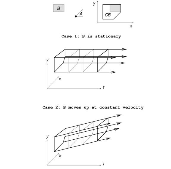
Each vertex of CBi traces out a curve in CT. The slope of this curve at any point gives the velocity of Bi at that point and its curvature gives the acceleration of Bi
Free space in CT defined as CTfree = CT\ U(CBi(t)). Its closure is called the semi-free space in CT.
A continuous map ξ : [0,1] -> CTfree is called a free CT-path
Problem reduced to finding a free CT-path between the two configuration times (qinit,0) and (qgoal,T). Hence reduced to finding a path among stationary obstacles, the CTBis
However, as already mentioned, need to make sure that the free path is time-monotone i.e. cannot go back in time. Thus the path should satisfy the condition: for all s, s' Є [0,1], let ξ(s) = (q, t) and ξ(s') = (q', t'); s < s' => t < t'.
for all s Є [0,1], ξ(s) = (q(t), t)
Path planning with moving obstacles believed to take time exponential in the number of moving obstacles
Reif and Sharir (1985) proved that dynamic motion planning in 3D workspace with arbitrarily many rotating obstacles is PSPACE-hard if the velocity modulus is bounded and NP-hard if the velocity modulus is unbounded
Canny (1988) showed that it is NP-hard to plan for a point robot with arbitrarily many obstacles, even if they are convex polygons moving at constant linear velocities
However, dynamic motion planning problem for a robot A translating at a fixed orientation in the plane with bounded velocity modulus among polygonal obstacles translating without rotation at a fixed speed can be solved in time polynomial in total no. of vertices of A and the Bis if the number of obstacles is bounded
General path planning algorithm by Schwarz and Sharir (1983) based on the Collin's decomposition (A cylindrical algebraic decomposition that is an exact decomposition of CTfree) used with a few changes to take care of monotonic behavior of time.
To account for the time monotonic constraint, configuration-time represented as a list (t,q1,....,qm) Є Rm+1 ( here m is the dimension of C) so that all cells ultimately project onto the time axis i.e. they are contained in "cylinders" above intervals or points along the time axis
Thus two cells are in the same cylinder or occur in the same interval of time if their sample points project at the same coordinate.
A directed connectivity graph built to ensure temporal ordering of cells. Thus the connectivity graph CG defined as a graph whose nodes are the cells of Collins decomposition of CT. A cell K is connected to a cell K' by a directed arc iff K and K' are adjacent and K occurs before or simultaneously with K'.
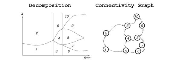
To generate a free path between (qinit,0) and (qgoal,T) the connectivity graph searched for a sequence of cells K1,....,Kp such that (qinit,0) Є K1 and (qgoal,T) Є Kp
However, slope of such a path with respect to time axis is not bounded and therefore the condition of the robot having unbounded velocity required.
If arrival time or the time when the robot is supposed to reach the goal is unspecified, then can use the same method. Here the goal locus is the half line { (qgoal,T) | T >= 0 }. In this case have to search for a path such that Kp intersects this line.
Above method is complete however impractical for even small values of m due to high computational complexity.
The Approximate Cell Decomposition approach using rectangloids used with a modification in the definition of the connectivity graph.
The connectivity graph CG defined as a directed graph whose nodes are the EMPTY cells (or both EMPTY and MIXED cells) of the decomposition. A cell K connected to a cell K' by a directed arc iff they are adjacent by a face parallel to the time axis or they are adjacent by a face perpendicular to the time-axis and K projects onto the time-axis before K'
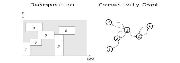
Planning is done by searching the connectivity graph for a sequence of adjacent cells forming an EMPTY or MIXED channel such that the first cell of the sequnce contains (qinit,0) and final cell contains (qgoal,T)
However the change introduced in the connectivity graph not enough to ensure that constructed channel contains strictly time-monotone CT-path.
This can be dealt with during graph searching by maintaining tearliest, the earliest time t which it can be in the current cell.
If the time interval on which the cell K projects itself on the time axis is considered to be [tmin(K),tmax(K)], tearliest can be computed as :
tearliest
= 0 at the start of the search
tearliest = max{ tearliest, tmin(K')} when
moving from a cell K to a cell K'
If currently in the cell K, cell K' can be chosen as next in the sequence iff there is an arc from K to K' in the connectivity graph and tearliest < tmax ( K' )
For C of given dimension m, time complexity increased as the algorithm is applied in m+1 dimensional CT-space however the constraint on the search reduces the size of the search space
The Approximate Cell Decomposition approach using rectangloids used in solving the motion planning problem with no velocity bounds can be further modified to solve the problem with bounded velocity. Concurrently with the generation of an EMPTY (or MIXED) channel, construct a time-monotone CT-path contained in this channel that satisfies the velocity constraint. One method is to discretize each cell of the channel into a grid of configuration-times and search the composite grid in the channel constructed so far. Therefore have to concurrently search the cell connectivity graph for a channel and the grid contained in the channel generated so far for a CT-path satisfying the velocity constraint. So, include a new cell in the channel only if a path can be extended to the new cell without violating the velocity constraint.
This method is not guaranteed to find a CT-path satisfying the velocity constraint in a channel even if one exists, due to discretization. Can be made more reliable however by discretizing the cells more finely, which results in an increase in computational cost.
A two phase approach to the dynamic motion planning problem. First plan a path for A from qinit to qgoal among stationary obstacles lying in W and then tuning the velocity of A along the path in order to avoid collisions with the moving obstacles. Thus problem broken down in to two sub-problems, the basic motion planning problem and the velocity-tuning problem
Velocity-tuning problem can be formulated as a dynamic motion planning problem in a path-time space similar to a two-dimensional configuration-time space.
Let τ : l Є [0,L] -> τ (l) Є C'free be the path planned in the first phase.
l is a parameter measuring the length of the path between τ (0) and τ (l) ( in the metric of C). Thus L is the total length of the path.
To generate a continuous function λ : t Є [0,T] -> λ(t) Є [0,L], with λ(0)=0 and
λ(T)=L, such that the composed map
τ o λ Є [0,T] -> τ(λ(t)) verifies (τ(λ(t)),t) Є CTfree for all t Є [0,T]. The map λ must be
such that A's velocity is bounded by Vmax. Also the function may not be
bijective so that it is possible for A to traverse some configuration in τ
more than once.
Let the lt-space [0,L]x[0,T] be called path-time space and be denoted by PT.
For a given path τ of A in C, a moving obstacle maps on to a region PTBi in this space called a PT-obstacle, defined as:
PTBi = {(l,t) Є [0,L]x[0,T] | τ (l) Є CBi(t) }
Let PTfree = [0,L]x[0,T]\U(PTBi)
Thus velocity tuning problem reduced to finding a strictly time-monotone continuous path in PTfree, called a free PT-path, between (0,0) and (L,T). This path determines a function λ which satisfies the given conditions i.e. (τ(λ(t)),t) Є CTfree for all t Є [0,T].
The slope of the PT-path with respect to time must also satisfy the velocity constraint, i.e. |dl/dt| < Vmax
Now, we assume that the PT-obstacles are polygons for simplification. This is the case when the path is a sequence of straight segments in C=R2 or R3 and the moving C-obstacles are polygons/polyhedra translating at constant linear velocities without rotation ( asteroid avoidance problem ).
Can use a variant of the visibility graph method to solve this problem which searches a refinement of the reduced visibility graph. The nodes of this directed graph are the convex vertices of the PT-obstacles and the two points (0,0) and (L,T). An arc of G connects the two nodes (l,t) to (l',t') iff t<t' and |(l'-l)/(t'-t)| < Vmax and either the line segment joining the two points is a PT-obstacle's edge, or it lies entirely in PTfree, except possibly at the endpoints where it is tangent to a PT-obstacle.
The velocity tuning approach is inherently incomplete. Given a path of A that avoids stationary obstacles, there may not be any velocity profile along that path which allows A to avoid collisions with moving obstacles.
However, this approach is more time-efficient than other methods. It is polynomial in the number of C-Obstacles and the total number of their vertices.
Here, we consider a collection of p robots, Ai, i = 1,...,p, moving in the same workspace W = RN, N=2 or 3, among stationary obstacles Bj , j=1,...,q. The robots move independently of each other, but cannot occupy the same space at the same time.
To plan a collision-free motion of the robots from an initial configuration to goal configuration i.e. generate p coordinated paths τi : [0,1] -> Cfree such that for all s in [0,1] no two Ai(τi(s)) and Aj(τj(s)) intersect.
The two major approaches used to solve this problem are:
Let C1,...,Cp be the individual configuration spaces of the p robots A1,..,Ap. Each Ci contains two sorts of C-obstacles:
C-obstacles of the second type are not static and depend on the motion of the robots.
The simplest way to extend the concept of configuration space to multiple robots is to consider the objects A1,..Ap as components of the same robot A = {A1,..,Ap}.
A configuration q of A is a specification of the position and orientation of
all frames FAi
attached to the robots Ai
with respect to the workspace frame Fw.
Since the robots move independently of each other , a configuration of A
is of the form q = {q1,...,qp}
where qi
denotes a configuration of Ai.
Thus A(q) = A(q1)
U A(q2)....
U A(qp)
and A's configuration space,
C = C1x....xCp
is called the composite configuration space of A1
through Ap.
It is a smooth manifold of the dimension m = sum of the dimensions of each of
the Ci's
C also contains two type of obstacles however they are time-independent.
CBij = { q = (q1,...,qp) Є C | Ai(qi) ∩ Bj ≠ Ф }
The C-obstacle corresponding to the collision of Ai with the robot Aj, i < j, denoted by CAij and defined by:
CAij = { q = (q1,...,qp) Є C | Ai(qi) ∩ Aj(qj) ≠ Ф }
Free space in C defined by: Cfree = C \ (U(CBij))U(U(CAij))
A free path between two configurations qinit and qgoal is a continuous map τ : [0,1] -> Cfree with τ(0) = qinit and τ(1) = qgoal
This is the approach which consists of planning the coordinated paths of multiple robots as a path in their composite configuration space. The projection of the path τ on every space Ci is the corresponding path of each robot Ai. The execution of the path τ requires that the individual robots follow their paths in a coordinated fashion. Changing the velocity of one robot requires the velocities of the other robots to be changed in the same ratio.
General path planning methods can be used for motion planning in the composite configuration space. Several specific methods have been developed to solve particular multi-robot motion planning problems.
Since C-space has a very high dimension ( ∑mi ), the time complexity is very high ( exponential in ∑mi ). Thus generally one of the RPP or PRM methods used.
J.C. Latombe. "Robot Motion Planning". Chapter 8
M. Erdman and T. Lozano-Perez. "On multiple moving objects". Algorithmica, 2:477-595, 1987
Y. K. Hwang. "Motion planning for multiple moving objects". Proc. of 1995 IEEE Symposium on Assembly and Task Planning (Local Copy)
B. Aronov, Mark de Berg, A. F. van der Stappen, P. Svestka, and J. Vleugels. "Motion Planning for Multiple Robots". Discrete & Computational Geometry 22:505--525, 1999 (Local Copy)
K.S. Hwang, H.J. Chao, and J.H. Lin. "Collision Avoidance Motion Planning amidst Multiple Moving Objects". 1999 (Local Copy)
Prof. Latombe's Robot Motion Planning Lecture Notes (Local Copy)