Rahul Erai
M Tech Computer Sc, IIT Kanpur
Kinect, PointClouds and PCL
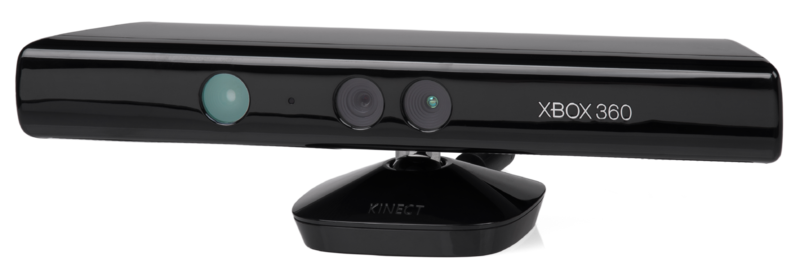
Kinect is a motion sensing input device by Microsoft for the Xbox 360 video game console. Using its infrared scanner and RGB camera, it can be used to capture 3D images(Well, actually 2.5D, since it can not capture data from the back side of the object scanned). It uses infrared structured light to get the 3D information.
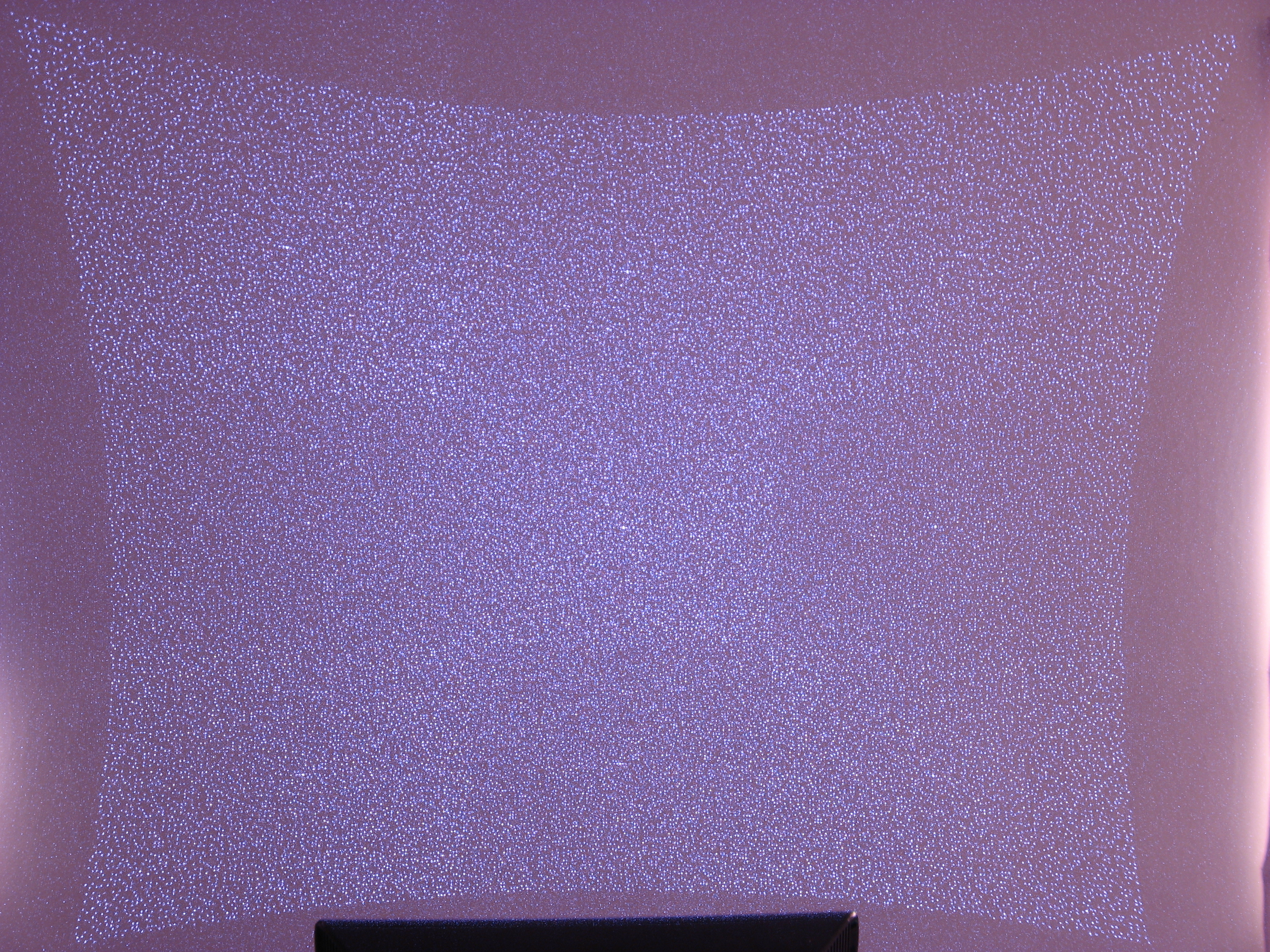
The IR emitter in the kinect throws a dot pattern, and based on the pattern reflected back, an extensively trained machine learning back-end calculates the shape and position of the object.
The IR scanner gives the depth information and the RGB camera gives the color
information. Once these are available and given camera calibration
parameters, one can can combine them together to form point cloud.
Point clouds are basically the 3D
counterpart of images, where instead of pixels, we have a set of points with X
Y and Z coordinate values (and possibly with additional information like color
and local normals).
In the right side, is the IR dot patterns emitted by the Kinect, captured
by a digital camera, whose IR cutoff filter is removed
[ Courtesy ].
The Point Cloud Library ,
better known as PCL, is a open source 3D point cloud processing library,
developed and maintained by Willow Garage.The PCL framework contains numerous
state-of-the art algorithms
including filtering, feature estimation, surface reconstruction, registration,
model fitting and segmentation.
Extracting object clusters from point clouds
One of the main challenge in visual perception is to extract the objects of interest from the background clutter. Compared to a 2D image, extracting objects from a 3D point cloud data is relatively simple, since we can make use of the one extra dimension. On the other hand, Kinect scans are very noisy, since its sole purpose was to use along with an gaming console. Nevertheless, I was able to extract objects from a relatively less cluttered environment. The high level structure of the algorithm used is shown in the block diagram bellow.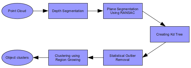
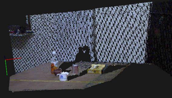
|
|
| Input point cloud | Results after RANSAC |
|
| Results after clustering |
Future works
Create some sort of signature for each object cluster, and try to track them in consecutive frames.VFHs, A signature for 3D Objects
In the last post, I explained how to segment and cluster objects in a noisy point cloud data. Now that we have the point clouds corresponding to the objects, the next task at hand is to derive some sort of unique signature for each 3D object, which can be used as means to detect and track these objects in a "3D point cloud video". One of such signature is Viewpoint Feature Histograms,or simply VFHs, introduced by Dr.Radu B Rusu and his team in 2010. First step in calculating VFH is to calulate central point of the object and surface normals at every point on the surface of the object. Then for the each point on the surface, calculate three parameters, which basically corresponds to the relative pan, tilt and yaw angle of the normal at the point, in a darboux frame coordinate system defined between the point and the center of the object. Once these three parameters are calculated for each point on the object, create an histogram out of it. This is the VFH signature of the object, and is fairly invariant to scale and rotation.
Dr. Rusu's paper on VFSs can be downloaded from here.
Results
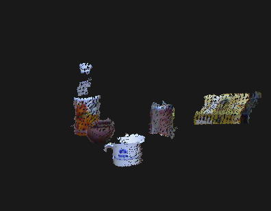
The input point cloud to the algorithm is shown bellow.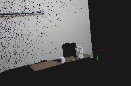
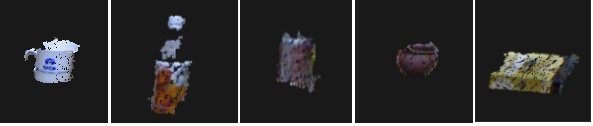
Then the objects in the cloud were segmented out by the techniques deiscribed in the previous post. Once the objects were seperated, VFH signatures were calculated for each of them. The segmented objects and their sigantures for two consicutive frames are given bellow.
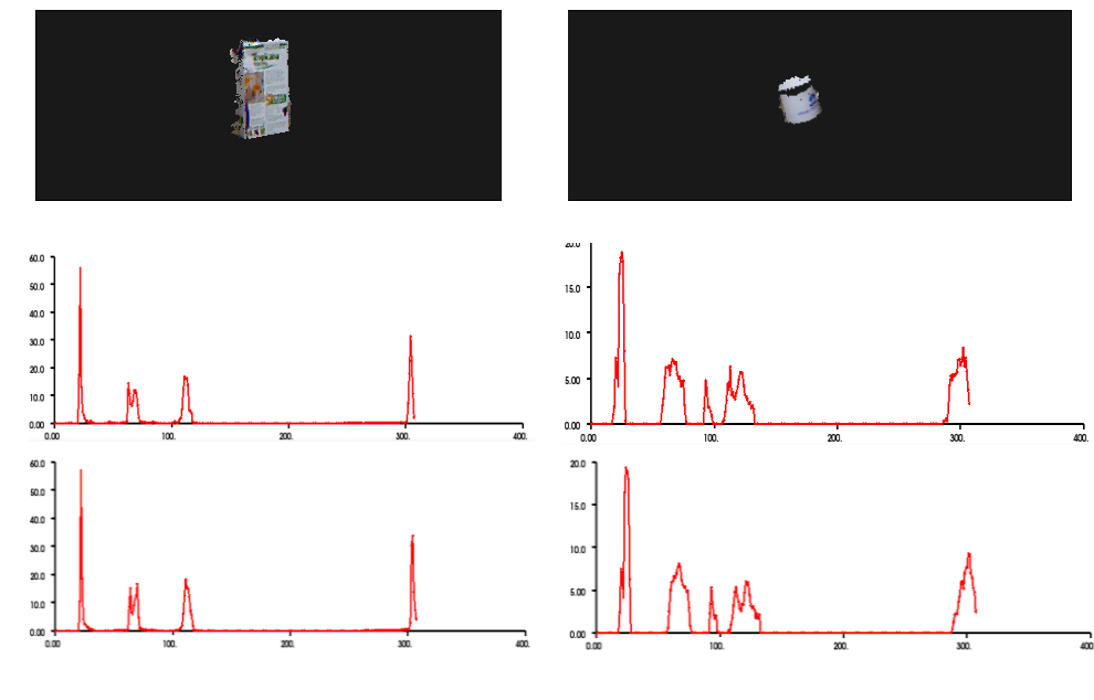
From the results given above, one can easily see that VFH signature of an object remains almost the same and can be used to uniquely identify objects in a cloud.
Future works
Now that we have calculated signatures for each object, the next step should be to use them in some object detection/tracking algorithm.Mapping Symbols to grounded Semantics
In last few posts, I've been discussing some of my efforts aimed at mimicking human visual perception using Kinect. But this post deals with the other end of the problem, mapping the learned information chunks to language. How does a human baby learns a language? It is well established that a baby learns "semantics" of a concept, long before he "labels" it with words in his mother tongue.In cognitive linguistics, these proto-concepts are known as image schemas. Once these schema are well established, baby begins to map the words uttered by elders around him to these grounded schemas. Later, more complex concepts are learned and labeled based on these grounded image schema. In this simple experiment, we tried to mimic this process.
The Experiment
This study was aimed at learning Malayalam labels corresponding to the concepts of tight and loose. The apparatus we used was a set of three small wooden planks with a hole on, and a set of 6 pegs with different sizes. Each of the three holes were associated with two pegs, among which one peg would go smoothly through the hole, while the other peg was pretty hard to insert in the hole. The picture of the apparatus is shown bellow.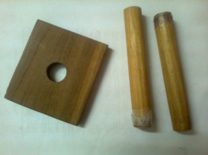
This apparatus were given to human subject, who were asked to insert these pegs to the holes, and describe the experience in unconstrained Malayalam. Three Malayalam speaking subjects were considered, and altogether 9 sets of commentaries were collected. Each set consisted of commentaries for a tight fit case and a loose fit case. Image schemas for tight and loose are assumed to be already available (Learning them would be comparatively simple, and can be done by training a neural network on sufficient number of holes and pegs). We are more interested in mapping words to these learned schemas.
One simple way of accomplishing this would be using conditional probabilities. Divide the commentaries into two sets, corresponding to loose fit trials and tight fit trials. Now for each word in either sets, calculate p(L/w); the probability that the word belongs to a loose fit experiment, and p(T/w); the probability that the word belongs to a tight fit experiment. The word that has to be associated with the concept loose should be w which maximizes p(L/w) / p(T/w). Similarly, the word associated with tight has to be p(T/w) / p(L/w). Assuming p(L) ~ p(T) and applying Bayes' rule, the ratio changes to p(w/L) / p(w/T) and p(w/T) / p(w/L) respectively.
Results
| Loose Trials | Tight Trials | |||||||||||||||||||||||||||||||
|
|
In loose trials, the word എളുപ്പത്തില് ranked first as expected, since it meaning loosely translates to "with ease". This makes sense, since in these trials, subjects were able to insert peg into holes with ease.
In tight trails, the word രണ്ടാമത്തെ came first, meaning "the second one". This was not the expected word. The reason for its appearance is that tight trials were always followed by the loose trails and subjects often uttered the word "രണ്ടാമത്തെ" in the second trial indicating that it was the second trial. Hence our classifier wrongly associated this with the concept of "tight". This could have been avoided by mixing up loose trials and tight trials arbitrarily while collecting the commentaries. The word ranked in the second position is സ്ടക്ക് , meaning "stuck, which accurately describes the trial.
Kinect RGB-D object dataset
I've been looking for a good benchmark dataset on kinect data to test my algorithms, and I finally found one. Washington University's RGB-D object dataset is an excellent dataset of pointclouds of household objects, captured using Kinect in a systematic way. The dataset comes with an excellent documentation, and is available free of cost on a request to the creators. Anyway, here goes a brief description of the dataset.
The dataset contains pointclouds, RGB images, and depth images of 51 categories of objects, captured by Kinect. The images are of 640x480 resolution, scanned at the rate of 30Hz. Apart from the main 51 categories, there are multiple instances of each object, hence the dataset can be used for instance detection as well.
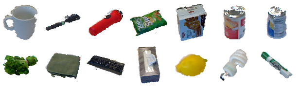
For each instance of an object, 3 video sequence were shot with kinect in three different heights, at approximately 30, 45 and 60 degree above the horizon, which captured the 360 degree views of the image. More information on the dataset can be found at this paper.
Testing Isomap on RGBD dataset
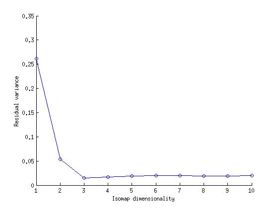
Isomap is a non-linear dimensionality reduction technique, which preserve the geodesic distance between the data points. More information can be found in this paper.
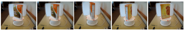
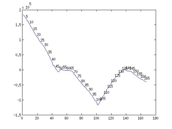
So when can one use Isomap based dimensionality reduction? Basically what Isomap does is that, it takes a manifold laying in a very high dimension, flatten it out, and maps to the desirable lower dimensional space. This preserves the geodesic distance, but the information about the shape/structure of the manifold is lost in the process. So in case of RGB-D dataset, the geodesic distance corresponds to the camera angle, since each object were shot in all 360 directions. Hence, if we apply Isomap to a 360 swipe of any object in the dataset, we can expect that the reduced data would be lying in 1-D.
Results
 |
 |
Object detection on RGB-D dataset
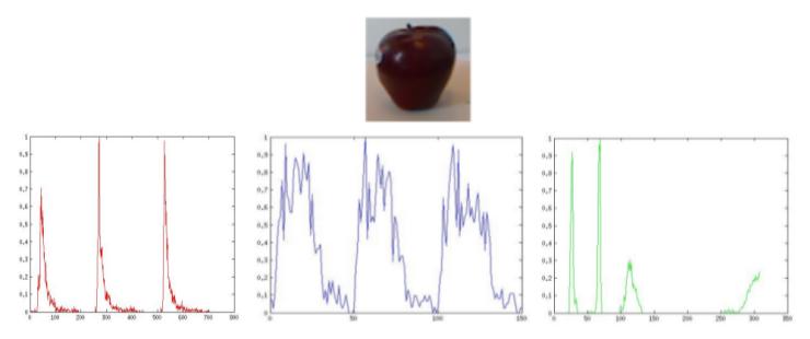
The first step in developing an object detection algorithm is to define a "signature" of an object, using which the object can be potentially differentiated from other similar objects. We already have discussed about VFH Signatures in one of the previous posts. They are signatures extracted from the 3D shape of the object. Using VFH alone may not give good results, since VFH doesn't contain any information about the texture and colour distribution of the object.
So we augmented VFH signature with two other histograms. The first one was a basic RGB histogram of bin size 256 x 3. This captured the global colour distribution of the object. The second histogram was based on SURF features. Usually, SURF features are calculated only at salient points in the image (at local maxima of first derivatives); but since objects in RGBD dataset are comparatively small and smooth, this may not be that useful. Alternatively, one find SURF points at EVERY point in the image, and it makes more sense since sometimes a lot SURF points with smaller SURF values would be more efficient in defining an object, than a few SURF points with high values. But we cant use all the SURF points as such as an signature, partly due to the high dimensionality of the resulting signature ( n x 64), and mainly due to the fact that number of SURF points would vary from object to object. An alternative would be, trying to capture how SURF points of an object are distributed in the 64 dimensional Euclidean space. A SURF distribution histogram that represent the same can be calculated as follows.
|
(i) Find the mean of all n SURF features. (ii) Calulate di for every SURF feature i. di is the distance between ith SURF feature and the mean. (iii) Bin all the di to 50 bins. |
So this SURF distribution histogram of red, green and blue components of the image would hopefully capture local texture distributions in the object. So our final signature is a 1226 dimensional vector, obtained by appending VFH histogram with an RGB histogram and a RGB SURF distribution histogram (all normalised between 0 and 1 separately).
Now that we have the signature, next step would be choosing a classification algorithm for classifying the objects based on the signature we created. We chose K-nearest neighbour as the standard algorithm, so that we can compare the results with future optimisations. There were 51 classes of objects. We left out one instance of the object from each class for testing, and used the images from all the remaining instances for training. This ensured that no image of the tested object were used for training.
Results
Over all detection rate : 54.43%|
Confusion matrix of 51 objects
|

|
Top 5 | Bottom 5 |
||||||||||||||||||||
|
|
Object detection on RGB-D dataset (IN REDUCED DIMENSION)
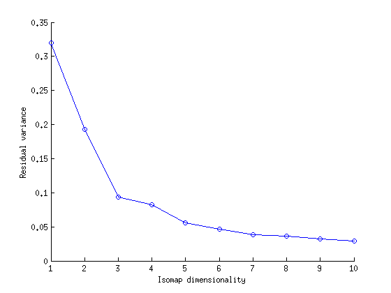
A croped object in RGB-D dataset is of the dimension 100x100x256x2 (~5,120,000). Hopefully, discriminating between the 51 categories in the RGB-D dataset could be done in a much lower dimension than 5 million. Here we investigate how much further one can reduce the dimension, with out reducing the detection rate. We would be using Isomap as the tool for dimensionality reduction.
The very first problem with using Isomap is that the dimensionality of the objects are not constant, since their cropped image size varies depending on the shape of the object. So we cant use raw rgb and depth images as such. Instead, we would be using the Object Siganturediscussed in the previous post as the starting point. Hence the dimensionality of the high-dimensional space is fixed to 1226, regardless the varying size of individual objects. Since a 360 degree sweep of each object is available, signature of an object couldn't't't change much between consecutive frames. Hence, even though the dimensionality of the space is 1226, objects should lie on a smooth lower dimensional manifold.
Results
KNN on raw data:euclidean, k=3 : 70.399%KNN on reduced dimensions (dim=10), k=9 : 69.018%
An unsupervised clustering algorithm for multiple manifold embedded space
One problem with above described isomap based dimensionality reduction technique is that, its performance is degraded if the space has multiple manifolds embedded in it. Isomap algorithm treats every point as te part of a single manifold, and tries to calculate geodesic distance between them. So, at the places were the manifolds are closer to each other, the graph grown through the manifold could jump from one manifold to another. One way to handle this situation would be using a small k as the branching factor of the graph being grown. This is not desirable due to two reason. Firstly, the value of k must be fixed according to the shape of the manifold one trying to encode, not the inter-manifold distance. Secondly, if one uses smaller value of k, the growth of the graph through the manifold can stop prematurely, breaking the manifolds apart. So one can not sole this problem with a constant k.One possible modification to the algorithm would be to change the way the graph grows through the manifold. Graph growing algorithm should be smart enough to bridge gaps in the manifold, without jumping to other neighbouring manifolds. This can be implemented by changing the branch factor of the graph dynamically. Instead of using a single k, we propose the use of two ks, k1,k2. K1 is the regular k, and should be set according to the expected shape of the manifolds. So this is the maximum degree of any vertex in the graph. K2 should be greater than K1,and should be directly prepositional to the expected size of gaps in the manifold. Now, assume at some vertex v, some of the k1 neighbours calculated are already visited. This might be probably happening because v is at the edge of the manifold, or near a gap in the manifold due to teh lack of proper sampling. Now,inclemently increase the branching factor from K1 to K2, till k1 un-visited points are obtained. If the algorithm fails to find k1 neighbours even after making the branch factor K2, one can assume that the vertex v was from the edge of the manifold. If it were near to a gap, the gap would have been bridged by the k2. Once the individual manifolds are identified, one can use isomap to embed each them separability into corresponding lower dimensions.
Enough with the theory, time to test it on our RGB-D datset. Considering the complexity of the isomap algorithm, we chose only the first 10 objects (alphabetically) from the dataset. So, our higher dimensional space contains atleast 10 manifolds. in reality, the number would be higher, since the instances of some objects varies alot(ie, green apple and red apple could lie in a separate manifold).
Results
Total number of input images : 10111Clustered images: 9651
Number of clusters : 100
Number of clusters with more than 90% purity: 77