3 Dimensional Voronoi Roadmap Methods

Introduction

Roadmap Methods for Robot Motion Planning rely on capturing the continuity of the robot's free space in a one-dimensional network of curves to which any point of the free space may be retracted. Once the roadmap is constructed, the problem reduces to joining the intial and goal positions to the roadmap and searching the roadmap for a path.

3D Voronoi Diagrams

Historical Background : Voronoi diagrams were first discussed by Peter Lejeune-Dirichlet in 1850.In 1908, the Russian Mathematician G. Voronoi wrote about them in a treatise on quadratic forms. They were earlier mentioned by Rene Descartes in the context of cosmic fragmentation in Part III of his Principia Philosophiae. They are also called Dirichlet regions, Thiessen polygons, or Wigner-Seitz cells. Dan Hoey suggested the more descriptive name proximal polygons for them.

Definitions

Given a set S={p₁, p₂,..., p_n},a Voronoi Polygon V(i) is the Locus of Proximity of points that are closer to a given point p_i than to any other point of S.

Generalized Voronoi Diagram : Given a set of geometric objects, or sites s1, s2, ..., sn, for each site si let a distance function di(x)=distance(si,x) be defined. The Voronoi region of si is the set V_i={x | d_i(x) < d_j(x), j!=i}.
The collection of regions V₁, V₂, ..., V_n is called the generalized Voronoi Diagram or GVD.

The term Voronoi diagram is varyingly used in literature to denote either the set of Voronoi polygons or alternatively their boundary. The boundary which is the locus of points equidistant to the two nearest sites, is also known as the medial axis. In the domain of Robot Motion Planning, we shall generally refer to this as the Voronoi Diagram.

For Robot Motion Planning problems, it is the GVD that is of interest for us.

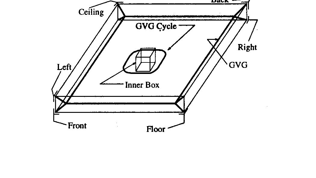
Generalized Voronoi Graph : Given a set of geometric objects, or sites s1,s2, ..., sn in m-dimensional space, the Generalized Voronoi Graph (GVG) is the locus of points equidistant from the m-nearest obstacles.A more mathematical definition would be :
The generalized Voronoi graph(GVG) is a graph embedded in R^m whose edges are m-equidistant faces and whose nodes are m+1 equidistant faces, m-boundary faces, and m-floating boundary faces.
A k-boundary face is the set of points on the boundary of the free space where k-obstacles intersect. In R^m, an (m-l) boundary face is termed the boundary edge and an m-boundary face is termed a boundary point, where the GVG edge and boundary edge meet.

A floating k-boundary face is the set of points in a k-equidistant face where at least two gradient vectors become collinear.

Dimensionality of the GVD and the GVG

In R^m, the GVD is (m-1) dimensional.When m=3 i.e in R³, the faces can be quadratic surfaces, the edges can be fourth degree curves and the vertices can be eigth degree algebraic points. This can be intuitively seen since :
--the locus of points equidistant from a point and a plane is a paraboloid.
--the locus of points equidistant from two lines is a hyperbolic sheet.

The GVG which is the locus of points equidistant to m nearest obstacles is 1-dimensional. A proof for this assertion is based on the pre-image theorem and uses the Equidistant Surface Transversality Assumption. The proof, being beyond the scope of this presentation, has been omitted. However at an intuitive level : consider a two-equidistant face F_ij ( a component of the GVD ). It is equidistant to the two nearest obstacles C_i and C_j.F_ij , F_jk and F_ik intersect to form an (m-2)-dimensional manifold that is equidistant to three obstacles. This procedure may be continued until a 1-dimensional structure is formed. Such a structure will be an m-equidistant face and is a one-dimensional set of points equidistant to m objects in m dimensions.

Hierarchial Generalized Voronoi Graph

In dimensions higher than two, the GVG is not guaranteed to be connected. An example of such a scenario in R³ is illustrated in the following figure.

Disconnected GVG

The generalized Voronoi regions and equidistant faces may be considered as a cellular decomposition of W into k-dimensional sets, where k=0, ..., m. If each k-dimensional cell is homeomorphic to a k-dimensional disk, then the one-dimensional cells of such a decomposition form a deformation retract or retract-like structure which is connected. The GVG in the figure is disconnected since the two-equidistant face corresponding to teh floor and ceiling of the room has a hole in between (due to the cubical box) and hence is not homeomorphic to a two-dimensional disk.Hence additional structures termed higher order generalized Voronoi graphs, need to be constructed in order to connect the GVG components. Higher order Voronoi graphs are basically GVG's defined on lower dimensional equidistant faces. As an example, in R³, a second order generalized Voronoi graph (GVG²) is analogous to a GVG that is restricted to a two-equidistant face.

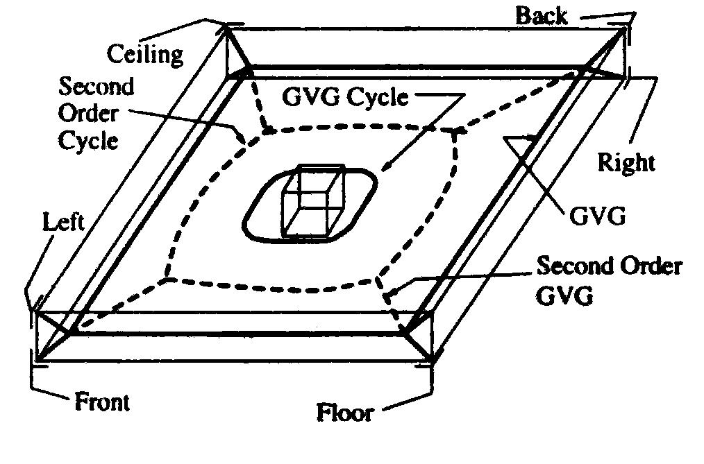
The Hierarchial Generalized Voronoi Graph (HGVG) is defined as the union of the GVG and all higher order generalized Voronoi graphs.

GVG² for a two-equidistant face ( drawn in dotted lines )

Incremental Construction of the HGVG

In this section an algorithm for incremental construction of the HGVG is described. This algorithm has eveolved at the Robotics Institute of CMU and forms the first step towards an ambitious plan of sensor-based motion planning for serpentine robots.The incremetal techniques used are such as provide a method for GVG construction using only line of sight sensory information. It is claimed by the developers that their techique can form the basis for a numerical method to construct a roadmap when the full geometry of the world is known in advance.

Incremetal Accessibility

The question under consideration here is whether a robot, given its intial position, can find its way to access the HGVG. Since the GVG is the major constituent of the HGVG, it suffices to show that the GVG possesses this property.A robot can access the GVG by following a path that is constructed using gradient ascent on the multi-object distance function D(x). D is not smooth and hence does not have a conventional gradient. However a generalized gradient may be defined as : genGrad(x)=Co{Del(d_i(x))} where Co denotes convex hull. It may be proved that if 0 belongs to the interior of genGrad(x) then x is a local maxima of D. This result, coupled with the following two lemmas are sufficient to conclude that if x is a local maxima of D, then it is equidistant to m+1 obstacles and hence lies on the GVG.Hence gradient ascent will bring the robot to a local maxima which lies on the GVG. Thus accessibility is assured.(Note : When Del(D) is a set, the vector with the smallest norm in Del(D) is chosen as the gradient).
Lemma 1 : Given a set of n arbitrary vectors in R^m, then 0 belongs to interior(Co{v_i belonging to R^m}) iff the set of vectors positively span R^m.
Lemma 2(Goldman and Tucker) : It requires a minimum of (m+1) vectors to positively span R^m.

Traceability

The approach followed uses techniques from numerical continuation methods which are used to trace roots of the equation G₁(y,lambda)=0 while varying lambda.In this context, let us look at the implicit function theorem and the Newton-Raphson Covergence Theorem without proof.

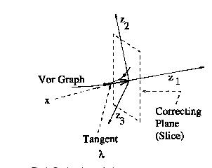
Let x be a point on the GVG. Choose local coordinates (z₁, ..., z_m) so that the first coordinate z₁ lies in the direction of the tangent to the graph.

Proposition : The tangent to a GVG edge at x is defined by the vector orthogonal to the hyperplane that contains the m closest points : c₁,...,c_m of the m closest obstacles C₁,...,C_{m.

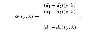
Thus the robot can obtain the tangent from local sensory data.}

We designate the hyperplane spanned by coordinates z₂,...,z_m as the normal slice plane. We then decompose the coordinates into x=(y,lambda) where lambda=z₁ is termed as the local sweep coordinate. We now define the function : G : R^m-1-›R X R^m-1 as follows :

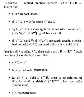
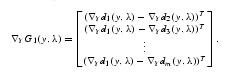
The function has a zero only on the GVG. Hence if the jacobian of G (given below) is surjective, then by the implicit function theorem, the roots of G(y,lambda) locally define a generalized Voronoi edge as lambda varies.

Assuming that the robot is currently at a point on the HGVG, it moves a distance delta(lambda) along the determined tangent direction i.e it predicts the next point to be traced. This prediction step causes some deviation of the robot from the GVG edge. Hence a correction step is followed. If delta(lambda) is small, the graph intersects a correcting plane which is parallel to the normal slice.

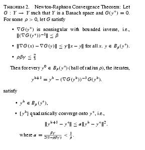
The correction procedure uses the iterative Newton's Method.The predicted position is used as an estimate and the correct root of the equation on the correcting plane is found. By the Newton-Raphson theorem, this iterative procedure is guaranteed to converge for our case.

Proposition : Given that equidistant faces transversally intersect in a bounded environment, if a generalized Voronoi edge is not a cycle, it must terminate : (1) at a generalized Voronoi vertex ( a meet point ), (2) on the boundary of the environment, or (3) at a point where two gradients of single object distance functions become collinear.

Incremental construction of the GVG proceeds in a fashion similar to graph search. Once the robot accesses the GVG, it begins tracing a GVG edge. On reaching a meet point it marks the direction from which it came as explored and then explores one of the other m edges, in the process also marking it. If the robot reaches another unvisited meet point, the procedure is recursively repeated.On reaching a boundary point or a floating boundary point, the robot turns around and retraces its path to some previous meet-point with unexplored directions. The robot continues its exploration till no more unexplored directions are left at any meet point. In case a specific destination is being sought, the robot may use a graph-search algorithm to control the tracing procedure.

Obtaining Distances and Gradients at a point

Distances to individual obstacles correspond to local minima in the robot's sensor array. The distance gradient is the unit vector pointing along the sensor measurement axis.

Detection of Meet Points

A meet point is a point at which the robot is equidistant to m+1 obstacles. However the robot's sensory information might not be accurate enough to exactly detect this condition. Besides, since the robot takes finite-sized steps, it might not pass exactly through a meet-point. Hence to robustly detect a meet point, the robot looks out for abrupt changes in directions of the (negated) gradients to the m-closest obstacles. Such a change implies that there is a meet point in the vicinity.

Departing from a Meet Point

At a meet point, the robot must be able to identify and xplore the m+1 GVG edges that emanate from it. If the robot wishes to trace the edge equidistant to obstacles C_i,...,C_m, proposition 1 ( stated above) may be used to obtain the 1D tangent space associated with that edge.Assuming v to be the computed tangent vector, the robot must decide whether to move along +v or -v. Let d₁)(x)=d₂(x)=...=d_m=d_m+1 be the distances. Then if del(d_m+1).v › del(d_i).v for all i in 1,...,m the the robot should move in the +v direction else in the -v direction.

Construction of GVG² Edges

Similar to the GVG edges, the GVG² edges are incrementally constructed by tracing roots of the equation :

while lambda is varied. Boundary edges may be traced by tracing the roots of the equation :

A floating boundary edge is a straight line and hence it is easy to trace.

Occluding edges

Occluding edges occur whenever a gradient to a minima defining an edge is interrupted by another object in its path.They are extremely difficult to trace. A cycle of occluding edges is detected by looking for discontinuities in the sensor readings of the robot as it traverses a boundary component of a second order region. A link is formed to the occluding cycle using gradient ascent(descent) of D. A cycle of boundary edges is detected in a similar fashion.

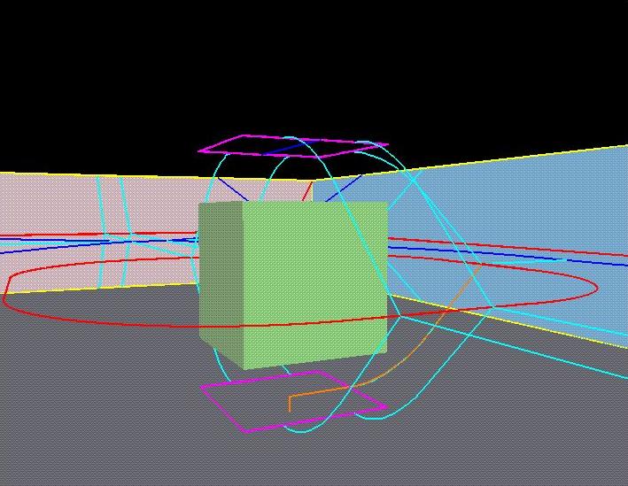
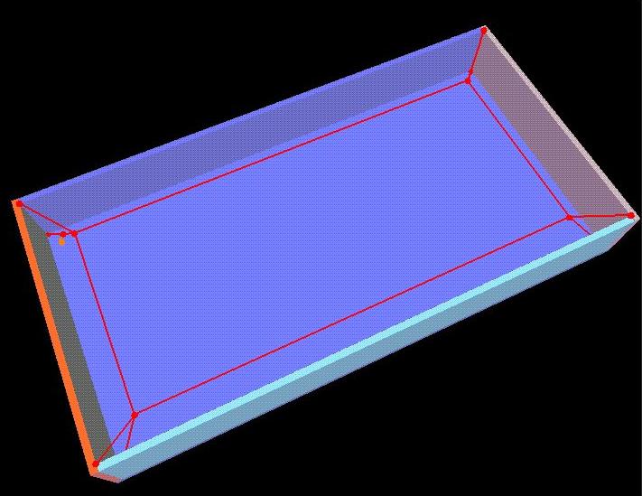
HGVG for a box floating in the centre of a rectangular enclosed room ( From : http://www.andrew.cmu.edu/~martin3/hgvgweb/faq.html )...occluded edges are shown in purple

Conclusion

The sensor-based motion planning approach outlined above is being developed chiefly at the Robotics Institute of CMU. It describes a motion planning methodology for a robot modeled as a point in higher-dimensional spaces. The chief focus is however on a three-dimensional space. Currently, research is on for obtaining a roadmap for a rod-robot. The researchers involved, state their eventual goal as the development of a roadmap for a chain of convex sets to model a highly articulated serpentine robot.

Links

HGVG Tracings obtained from 3D Simulator at CMU
HGVG in a nutshell (CMU)
HGVG for Rod-Shaped Robots
Papers on the GVG/HGVG

References

Preparata, F.P and M.I Shamos (1985) Computational Geometry : An Introduction, Springer-Verlag, New York.
Choset H. Incremental Construction of the Generalized Voronoi Diagram, the Generalized Voronoi Graph, and the Hierarchial Generalized Voronoi Graph.
Choset H. and J. Burdick,Sensor Based Motion Planning : The Hierarchial Generalized Voronoi Graph.
Choset et al, Sensor-Based Exploration:Incremental Construction of the Hierarchial Generalized Voronoi Graph,The International Journal of Robotics Research, February 2000. ( Locally Cached Copy )