SE367
HW4
Vidur Kumar (Y8560)
Q1.
a) Plot of residual errors versus the no. of dimensions chosen (for 100 images)
 ResidualVariance_vs_IsomapDimension.png)
b) The variance is minimal when there are two dimensions chosen for the isomap- most likely because the data is best represented in two dimensions.
This is further corroborated by the fact that increasing the number of dimensions of the isomap, to more than two, does not alter the residual variance at all. Infact, if anything, it is infinitesimally increased with increasing dimensions of the isomap - the only plausible explanation for which could be the addition of noise with the inclusion of unnecessary dimensions.
c) Plot of the 2D Isomap with labelled boundary points of (Theta1) and (Theta2):
 2D Isomap embedding (with neighborhood graph) - Copy.png)
As it is seen from the above labelling of the plot - the occurance of theta-boundary points are not in any particular patterns in the Isomap. Nor do all points on the boundary of the Isomap represent boundary points of theta.
Hence, it is assumed that there is no pattern in relating the plots of the Isomap representation of the vectors with that in Eucledian space.
d) Plot of residual errors for 2D Isomap generation over 1000 images :
 ResidualVariance.png)
The residual error shows a similar pattern as seen for the Isomap generated for 100 images - with the only variation being that the absolute value of the error has gone down, by virtue of the larger number of data points to choose the eigen vectors more precisely.
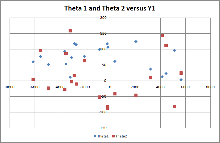
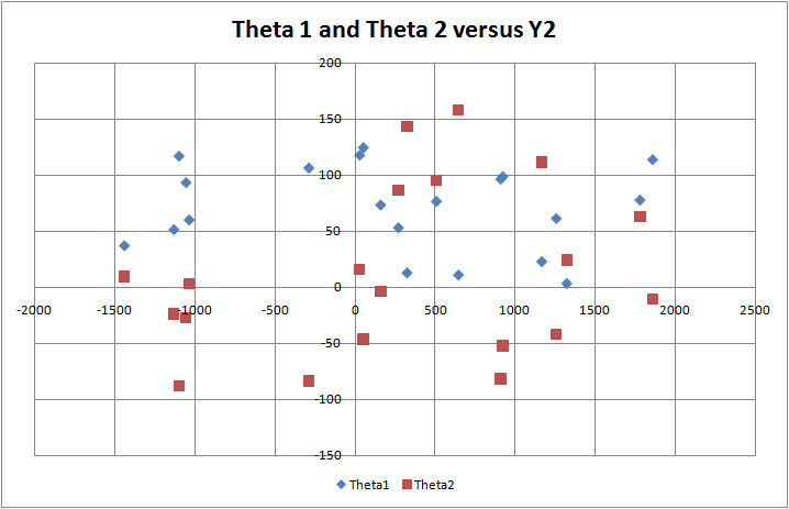
e) The values of Y1 and Y2 versus Theta1 and Theta2, which have been plotted as shown :
| Y1 | Y2 | Theta1 | Theta2 | |
| 1 | 4446.367685 | 1164.778935 | 23.061785 | 111.920576 |
| 2 | 4134.200528 | 323.6929394 | 13.010174 | 143.673573 |
| 3 | -2052.107757 | 1777.2488 | 77.935974 | 63.507889 |
| 4 | -3621.799525 | -1054.84844 | 93.446213 | -27.068283 |
| 5 | -2861.849756 | 28.53883074 | 117.977051 | 16.14006 |
| 6 | -6139.902964 | -1035.405504 | 60.216198 | 3.45488 |
| 7 | -862.8480584 | 921.5577661 | 98.890152 | -52.05019 |
| 8 | -3520.120481 | 270.0209506 | 53.22966 | 86.592529 |
| 9 | -2700.068712 | 1856.022592 | 114.079742 | -10.437866 |
| 10 | 5113.083798 | 907.9178429 | 96.59771 | -81.656945 |
| 11 | 371.2288524 | 1255.061606 | 61.536392 | -41.745966 |
| 12 | -3068.718884 | 159.2593573 | 73.605782 | -3.282196 |
| 13 | -5542.463144 | 507.3439305 | 76.759033 | 95.872925 |
| 14 | -232.9344764 | -1098.584115 | 117.142075 | -87.767963 |
| 15 | 3208.814481 | -1439.483843 | 37.193707 | 9.671291 |
| 16 | 2045.998808 | 51.52377313 | 124.752792 | -46.28672 |
| 17 | -182.8565163 | -288.9544859 | 106.577217 | -83.606153 |
| 18 | -3190.656936 | 644.9811566 | 11.097768 | 158.217799 |
| 19 | 5638.949873 | 1320.331654 | 3.452615 | 24.305352 |
| 20 | -4927.76027 | -1130.816218 | 51.594627 | -23.742022 |
The plot of (Theta 1 and Theta 2) vs Y1 and Y2 respectively - did not yield any significant patterns (atleast in terms of linear-fits).
Q2.
The eigen values for the PCA analysis (for 10dimensions) are as follows :
951682.4
402869.8
332749.8
102007.5
71759.04
43769.68
28116.36
21325.43
17958.51
16813.90
Hence, it is visible that the first two are not very significantly greater than the other eigen values - which should ideally reflect in the quality of the reconstruction, but does not seem to be affecting the image in any significant way (considering the angles theta1 and theta2):
PCA-Reconstruction, using 2 eigen vectors:
 PCA-Reconstruction, using 10 eigen vectors:
Q3.
a) Reconstruction of the x' vector (corresponding to y' vector in eigen space - after LLE reduction of the vector/image-space) :
b) Reconstruction of x', corresponding to y' vector (after Isomap-algorithm based reduction of vector/image-space) [taking the weightage function for the local neighbours]:
.png)
Reconstruction after PCA (taking 2-eigen vectors) - (given above as well)
c) From the above examples - it is clearly visible that the reconstruction of y-data (in eigen space) back to its x-data-form (original dimensional space), is best facilitated when utilizing the original-data of the neighbouring points (which are calculated in the eigen space).
This is so - since using the original data, with weightage functions, allows for the inclusion of all details that existed in the original dimensions - as opposed to attempting to reconstruct the data from a linear expression of the eigen vectors in a linear space - specially when the no. of eigen vectors chosen is fewer than the dimension order of the original vector/image-space.
The eigen vectors allow for a resemblence to original data, upon reconstruction - because the 'constant' or non-variable data, is adjusted for within the chosen eigen-vectors that define the lower-dimensional eigen-space.. Hence, reconstructing from that coordinates in the eigen space, back to the original space - results in images that resemble the original image, but still lose out on some of the details.
The linear systems are more simplistic in their deconstruction/dimension-reduction methodology - and also in their reconstruction methodology - but do therefore, also allow for a greater loss of data, for the same degree of information retained (in terms of stored space in bytes). Their data is stored in terms of the coordinates in eigen space, and the representation of the eigen vectors in the original vector/image space.
The non-linear systems are more complex in their construction and deconstruction algorithms - but give far better results, for the same amount of information being stored. Their data is stored as a set of nodes and geodesic distances between nodes.
NOTE - the data in the non-linear system is stored as a function of the local neighbourhood of points - within which it is linear. Hence, resulting in multiple pockets of linearity, that allow for overall reduction of data by following the distances along these linear neighbourhoods (from one neighbourhood to another - and hence, traversing the entire image-space)- but there is no global linearity in the storage.
Q4.
Having run the Isomap and PCA algorithm on the set of 2000images, it can be said that the non-linear method is more efficient than the linear method - since it does not assume or require a pattern or a particular distrubtion in the vector/image-space, for it to give efficient reconstructions.
The linear methods are less efficient, since they are effective (in dimensions reduction) only if the data in the vector/image space, is oriented suitable for that reduction.
The linear methods have the advantage in being faster and requiring less processing - but suffer from the loss of efficiency in reconstruction, even when using the neighbours to do the reconstruction.
Example :
PCA-reconstructed image (using neighbours)
 PCA reconstruction (nhgbrs).png)
The more intense image in the reconstruction does not match the theta-angles of the two images taken to creat this new averaged image - while the shadow-image's angles do match the average of the two thetas.
This is probably explainable as the fact that since the y1,y2 did not map in any particular pattern to theta1,theta2 - therefore, in the eigen space - the neighbours of the overaged y1,y2 point - came out to be those with a great deviation in theta1,theta2. Hence, the image is grossly inaccurate to what it should be
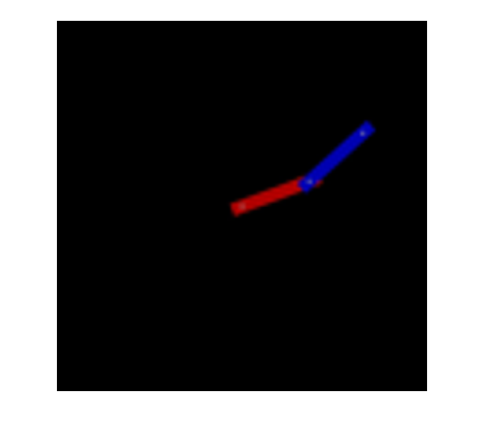
IMAGE : Isomap reconstruction using neighbours:
 ISOMAP reconstruction (nhgbrs).png)
This image is the accurate average of the two images whose average was taken to create this piont in the representation space.
HENCE - non-linear methods do seem to have the edge over linear methods.