Matlab code files(.zip) - Code
(a)
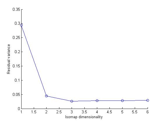
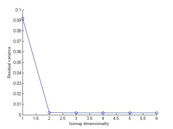
(b)We look for an elbow in the graph after which the residual variance doesnt decrease significantly after adding dimensions. For the given data, there is an elbow at d=2, which is also the known dimensionality of the data set(theta1, theta2).
(c)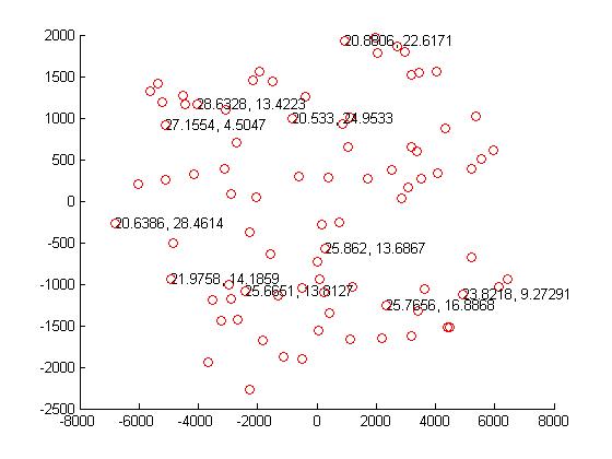
The boundary values for theta1 are at the boundaries of the 2-D plot; lowest being on the left and highest on the top right. For theta2, the boundary values, both highest and lowest occur together on the top left of the plot.
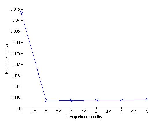
(d)The graph of residual variances vs dimensionality obeys the same shape, but the variances when the input is of 1k files are larger. Here is the graph for a comparison:
(e)Table:
theta1 theta2 y1 y2
1.0e+003 *
0.0217 0.0233 -4.4464 1.1648
0.0210 0.0264 -4.1342 0.3237
0.0258 0.0199 2.0521 1.7772
0.0269 0.0105 3.6218 -1.0548
0.0287 0.0162 2.8618 0.0285
0.0245 0.0126 6.1399 -1.0354
0.0273 0.0079 0.8628 0.9216
0.0239 0.0216 3.5201 0.2700
0.0285 0.0131 2.7001 1.8560
0.0272 0.0045 -5.1131 0.9079
0.0246 0.0076 -0.3712 1.2551
0.0255 0.0124 3.0687 0.1593
0.0257 0.0235 5.5425 0.5073
0.0287 0.0046 0.2329 -1.0986
0.0228 0.0125 -3.2088 -1.4395
0.0292 0.0095 -2.0460 0.0515
0.0279 0.0047 0.1829 -0.2890
0.0208 0.0280 3.1907 0.6450
0.0203 0.0128 -5.6389 1.3203
0.0238 0.0093 4.9278 -1.1308
A clear gradation of the values of theta1 with y1 cant be seen, nor with y2. Similarly, for theta2. As such, it doesnt seem likely that theta1, theta2 could be mapped to y1, y2.
The contribution to the variance from the top two eigenvectors is 63.41% and 18.65% respectively. They together contribute more than 80% to the total variance!
I was able to apply LLE to the image data, however, wasnt able to reconstruct the images from the lle and isomap data.