(1)
(a) Show the graph of the residual error vs dimensions for random100.zip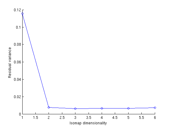 | (b) Discuss the result you find. Broadly , the error of embedding decreases with increasing dimensionality. But there is a sharp decrease from D = 1 to D = 2 when error drops from .15 to .02. Whereas from 2 to 6 dimensions the error is somewhat constant. Thus, out dataset can be parametrized in 2 dimensions |
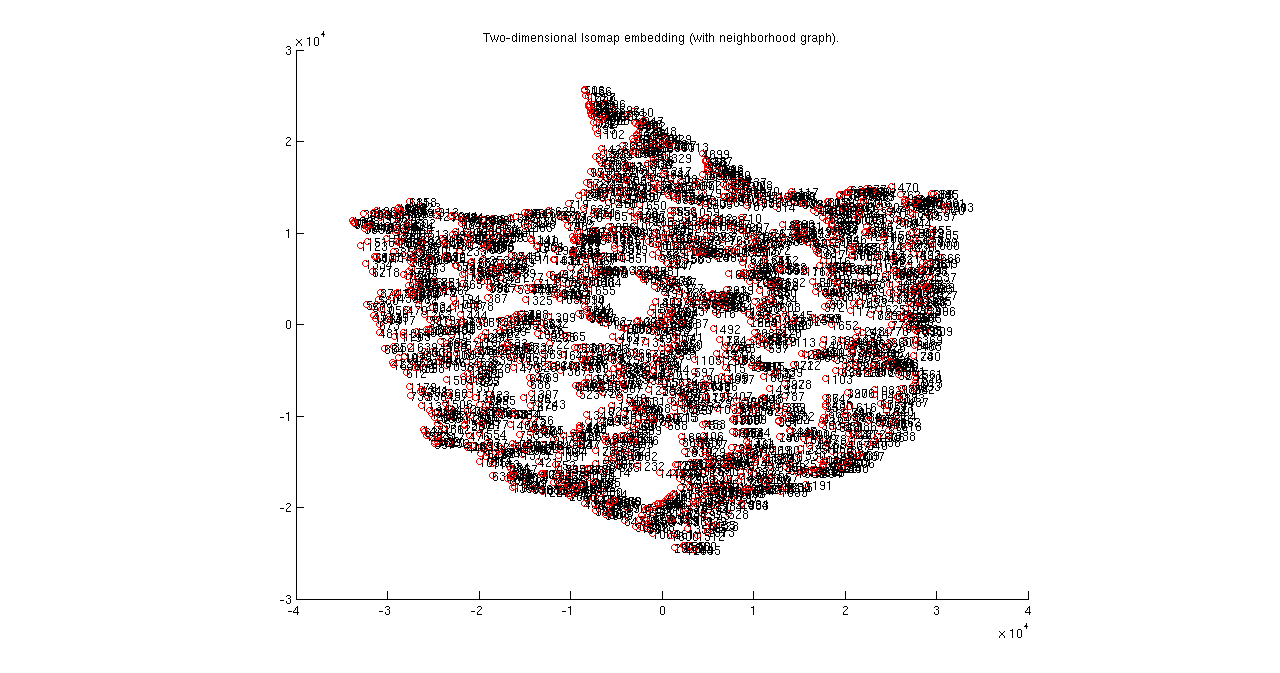
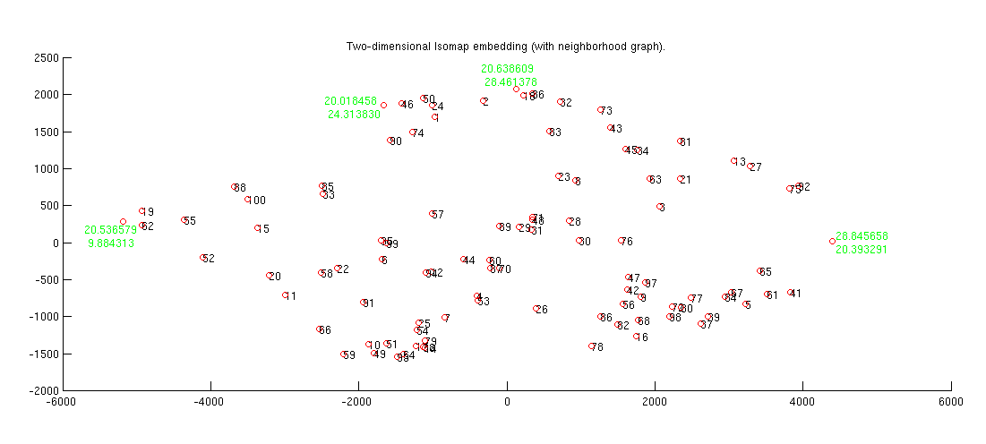
(c) In the 2-D mapping, a graph is generated. Label some of the points in this mapping with the theta1,theta2 in the textfile. Are the boundary thetas at the boundaries of the 2D-patch?
We have replaced four points in Isomap with their coordinates and in those points there is no correlation between edges of theta1 and theta2
| 
|
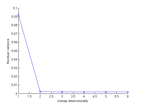
(d) When we compute this graph on the images in randomMotion1K.zip, how do the residual errors change?
As we can see in the adjoining plot and table below errors have decreased when we used 1K images.
Dimensionality | 1K images | 100 images | 1 2 3 4 5 6 | 0.092076 0.0021925 0.0018417 0.001772 0.0017997 0.0020052 | 0.11567 0.0075598 0.0063086 0.0065472 0.0066643 0.0070606 |
| 
|
(e) Give a table of the first 20 theta1 theta2 vs y1 y2 (Isomap) What can you say about mapping these y to theta1 and theta2 of the arm?
Theta 1 | Theta 2 | Isomap 1 | Isomap 2 |
|
21.70828 20.963717 25.773035 26.921942 28.73904 24.460459 27.325196 23.942938 28.450352 27.155386 24.558251 25.45228 25.685854 28.677191 22.755089 29.240948 27.894608 20.822057 20.255749 23.821824 | 23.289759 26.445587 19.94295 10.453383 16.162862 12.614105 7.879244 21.592861 13.065413 4.504699 7.640685 12.361451 23.495475 4.586599 12.452133 9.477505 4.657732 27.990783 12.828469 9.27291 | -968.969672131827 -320.964651530104 2059.15121123434 -407.751715206392 3222.90273577482 -1682.74536695542 -836.696315507224 930.7107681178 1804.10460193679 -1865.34476288468 -2989.25802394521 -1018.05481832057 3063.78645093637 -1106.49965959172 -3374.06213889779 1752.05010314218 -1223.87831444555 221.336745807909 -4929.55276950792 -3216.05372641485 | -1704.91448153208 -1916.58777619462 -486.005247478678 722.82679471592 826.013532204066 223.741840571482 1008.25810136635 -845.812499694978 732.864507797734 1371.86693533614 705.690844778986 389.61336323464 -1103.81884781531 1420.23002127535 -196.461511353476 1257.70260679073 1395.12212528639 -1995.18934366587 -431.205866608188 441.99719887198 | 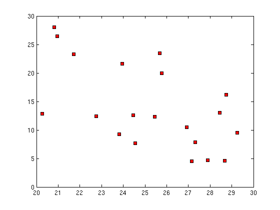 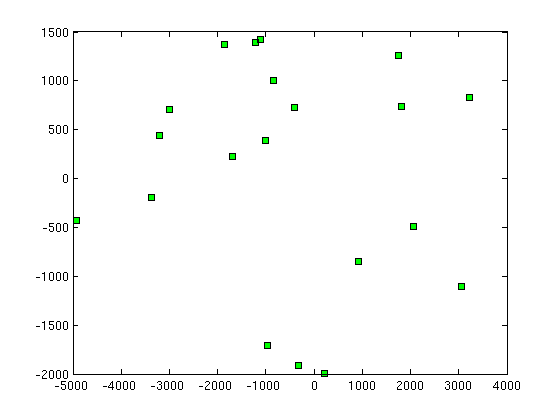
As we can see from above plots of theta1 vs theta2 and isomap1 vs isomap2, if there is any correlation between them, it cannot be visualised easily. But we can see that each of the plots can be divided into 3-4 clusters and these clusters can be individually mapped from (t1, t2) to (isomap1,isomap2) |
(2) Use PCA on randomMotion100.zip to map it to 2 dimensions (keep the top two eigenvalues). How much larger are these two eigenvalues compared to the others
Top two eigenvalues are : 23294 and 3166 and they are very large as compared to remaining eigenvalues. In decreasing order other eigenvalues are 1334, 1005 and 322 and so on.
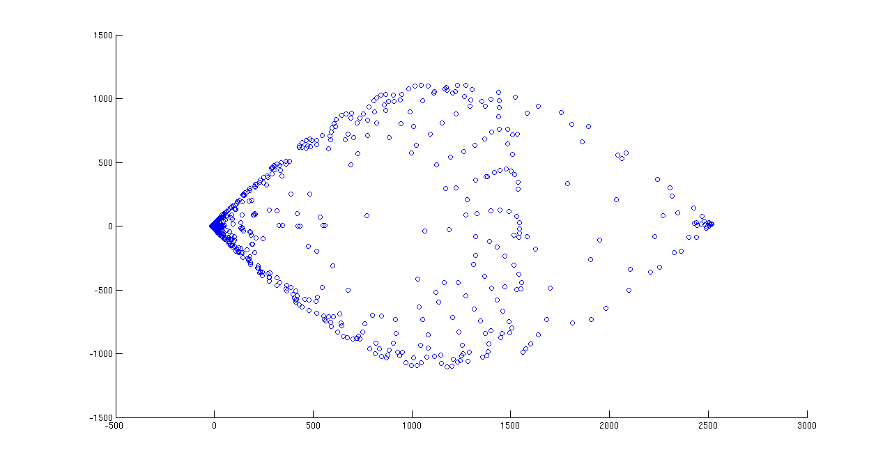
PCA scatter plot on 100 images drawn using matlab’s scatter and princomp function {[pc, zscores, pcvars] = princomp(double(data)); scatter(zscores(:,1),zscores(:,2));}
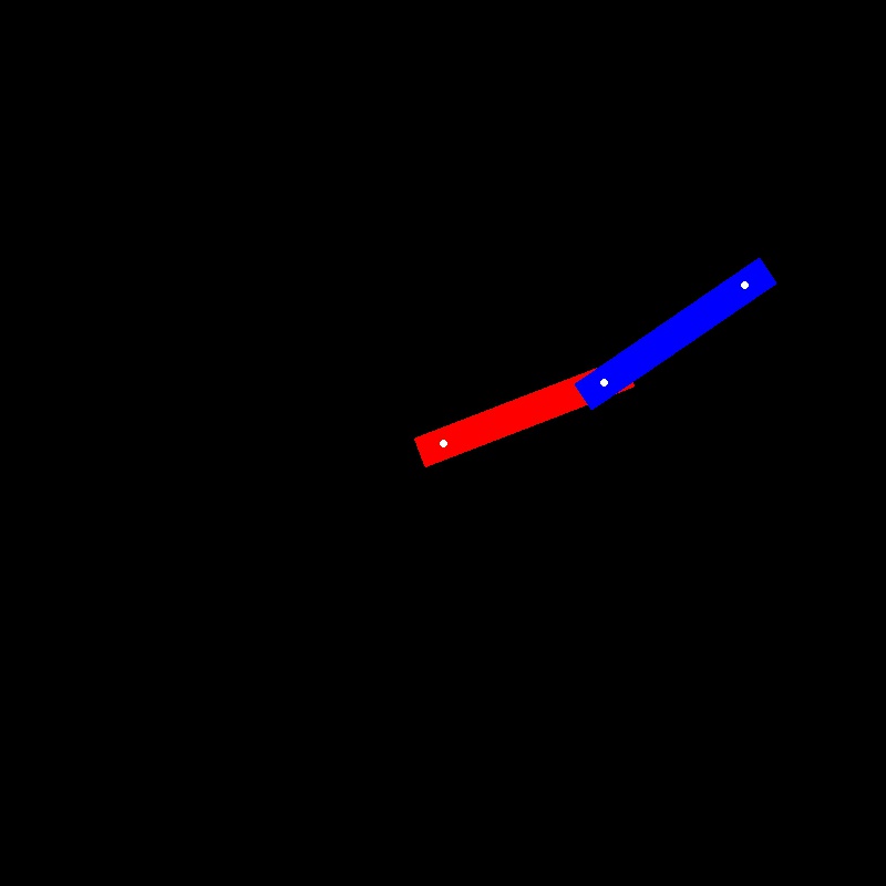
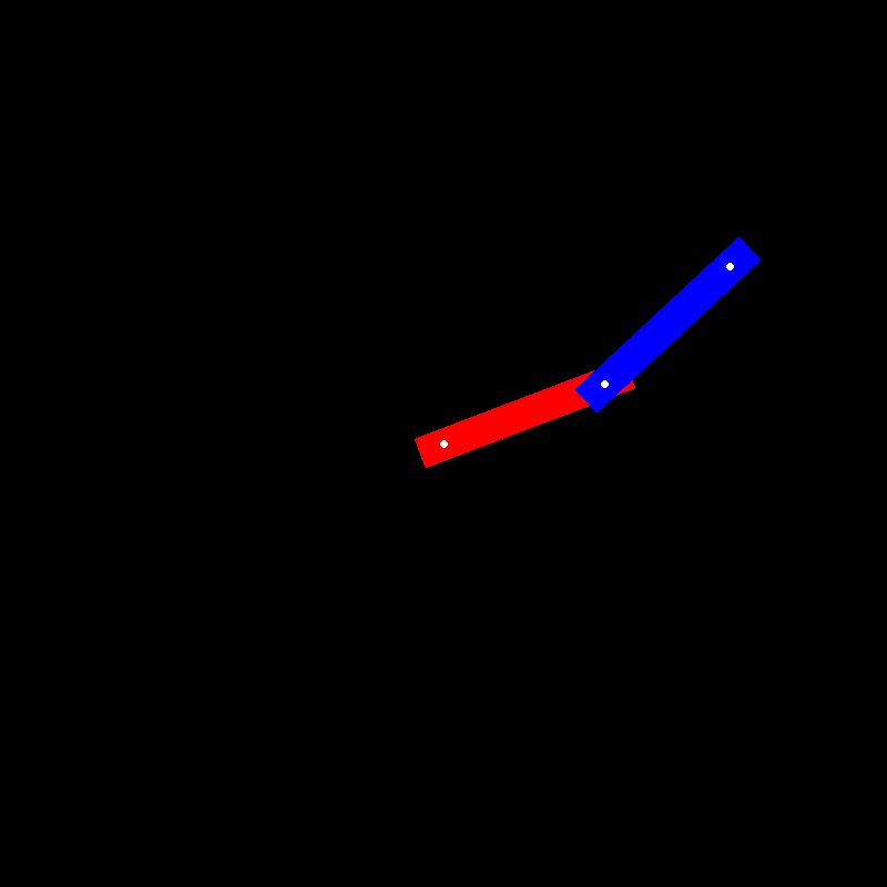
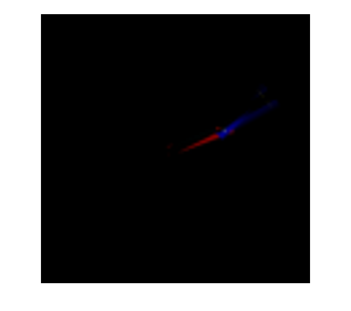
image 1 in dataset | image 2 in dataset | Reconstructed image from PCA |
Matlab code :
[mappedX, mapping] = pca(double(data'), 2); % pca, mixed integer types not allowed , converted to double
mean_elem12 = (mappedX(1,:) + mappedX(2,:))/2; % find mean of 1st and 2nd sample from images
mapped_elem12 = mean_elem12*mapping.M'; % backmap/reconstruct
to_image = imresize(uint8(reshape(mapped_elem12, 100, 100,3)),[800 800]); % make image
(3) Non-Linear mapping and reconstruction:
LLE: Use Local Linear Embedding to map the data to 2D. Now for the same point y', obtain the original image x'. In this case, you will need to find a set of closest neighbours yj (in 2D) and interpolate between them (express y' = SUM wj yj). Now, in image space, knowing the mapping xj for each yj, find x' = SUM wj xj.
Matlab code :
mappedX = lle(single(A'),2);
mean_elem12 = (mappedX(1,:) + mappedX(2,:))/2; % find mean of 1st and 2nd sample from images
neighbours_elem12 = knnsearch(mappedX, mean_elem12,'K', 5); % use knnsearch with 5 neeighbours
weights = mappedX(neighbours_elem12,:)'\mean_elem12' % find weights for each neighbours
mapped_elem12 = weights'*single(A(:,neighbours_elem12)'); % find backmaps
to_image = imresize(uint8(reshape(mapped_elem12, 100, 100,3)),[800 800]); % make image
Use the same idea of local linearity to do the reconstruction in the ISOMAP case. Draw the reconstruction x'.
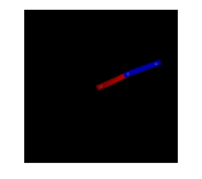
Reconstructed image from PCA | image 2 in dataset | image 1 in dataset |
(4) In completeMotion2K.zip, we cconsider a full range of motion (theta1 = 0 to 135 degrees, theta2 = 0 to 180 degrees). Apply PCA and Isomap to the data, for d=2. What can you say about the effectiveness of linear vs nonlinear methods for this task?