End to End
properties means:
Everything is measured at the 2 ends of the connection. The internet is considered as a black box.
How the properties are measured?
The properties are measured using tcp traces.
The advantages are :
1: The tcp traces are directly indicative of the TCP performance.This is because the TCP
traffic is "real world" as it is widely used in today's Internet.Consequently any network path
properties that we can derive from measurements of TCP transfer can potentially be directly applied to
tuning TCP performance.
2: TCP packet streams allow fine-scale probing without unduly loading the network,
since TCP adapts its transmission rate to current congestion levels.
The disadvantages are:
1: we need to distinguish between the apparently intertwined effects of the transport protocol
and the network.
2: TCP packets are sent over a wide range of time scales, from milliseconds to many seconds between
consecutive packets.Such irregular spacing greatly complicates correlational and frequency-domain analysis, because a stream of TCP packets does not give us a traditional time series of constant-rate observations to work with.
More on setup
This study of internet packet dynamics was conducted by tracing 20,000 TCP bulk transfers
between 35 Internet sites.
These sites run special measurement daemons i.e NPDs to facilitate measurement.With this framework the number of internet paths avaliable for measurement grows as N2(N square) for N sites yielding attractive scaling.
The first run N1 was conducted December 1994 and the second run N2 during Nov-Dec 1995.
The differences between N1 and N2 give an indication of how Internet Packet dyanamics changed during the course of 1995.
Each measurement was made by instructing daemons running at two of the sites to send or recieve a 100 Kbyte TCP bulk transfer and to trace the results using tcpdump.
Measurements occurred at Poisson intervals,which, in principle, results in unbiased measurement,
even if the sampling rate varies .
In N1 the the mean per-site sampling interval was about 2 hours, with each site randomly
paired with another.
In N2 sampling was done onpairs of sitres in a series of grouped measurements varying the sampling
rate from minutes to days, with most rates on the order of 4-30 minutes.
These groups then give observations of the path between the site pair over a wide range
of time scales.
Another difference between N1 and N2 was that in N2 Unox Sockets were used to assure that the sending and
the receiving Tcps had big windows to prevent window limitations from throttling the transfer's throughput.
The properties which measured were:
Packet reordering
Even though Internet routers employ FIFO queueing, any time a route changes, if the new route offers a lower delay
than the old one, then reordering can occur.
Detection of reordering
The reordered packets were recorded at both end of each TCP connection. Any Trace pairs suffering filter errors were removed.
Then for each arriving packet pi it is checked whether it was sent after the non-reordered packet.If so it becomes the new such packet .
Otherwise it's arrival is counted as an instance of network reordering.
Observations of reordering
There was significant amount of reordering. Overall there was 2% of all of the N1 data packets and 0.6% of the acks arrived out of order.
For N2 it was 0.3% of all data packets and 0.1% of acks. Thus the data packets were reordered more than the acks.
It was aslso observed that the out-of-order delivery varies from site to site .For e.g for the "ucol" site 15% of the data were reordered much higher
than the 2.0% average.
Also reordering was highly asymmetric. Only 1.5% of the data packets sent to ucol during N1 arrived out of order.
Thus, we should not interpret the prevalence of out-oforder delivery summarized above as giving representative
numbers for the Internet, but instead form the rule of thumb: Internet paths are sometimes subject to a high incidence of reordering, but the effect is strongly site-dependent, and apparently correlated with route fluttering, which makes sense since route fluttering provides a mechanism for frequently reordering packets.
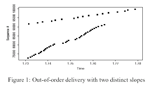
Figure shows a sequence plot exhibiting a massive reordering event. This plot reflects packet arrivals at the TCP receiver, where each
square marks the upper sequence number of an arriving data packet. All packets were sent in increasing sequence order. Fitting a line to the
upper points yields a data rate of a little over 170 Kbyte/sec, which was indeed the true (T1) bottleneck rate ( 4). The slope of the packets
delivered late,though, is just under 1 Mbyte/sec, consistent with an Ethernet bottleneck. What has apparently happened is that a router with
Ethernet-limited connectivity to the receiver stopped forwarding packets for 110 msec just as sequence 72,705 arrived,most likely because at that point it processed a routing update. It finished between the arrival of 91,137 and 91,649, and began forwarding packets normally again at their
arrival rate, namely T1 speed. Meanwhile, it had queued 35 packets while processing the update, and these it now finally forwarded whenever it
had a chance, so they went out as quickly as possible, namely at Ethernet speed, but interspersed with newarrivals.
This pattern was observed a number of times not frequent enough to conclude it is anything but a pathology,but often enough to suggest that
significant momentary increases in networking delay can be due to effects different from both route changes and queuing most likely due to
forwarding lulls.
Effect of reordering
While out of order delivery can violate one's assumption about the network,the abstraction i.e well modelled as a series of FIFO queing servers
it was found that it had little impact on TCP performance.
The value of duplicate threshold Nd =3 was choosen primarily to assure the threshold e\was conservative.
Two possible ways to improve fast retransmit mechanism:
1:>By delaying the generation of dups to better idsambiguate packet loss from reordering and
2:>By altering threshold to improve the balance between seizing retransmission oportunities verses avoiding unneeded transmissions.
Packet reordering time scales:
The presence of spikes was found strongest at 81ms.
For N1 20ms would identify 70% of out of order deliveries.
For N2 8ms would identify 70% of out of order deliveries.
Thus a generally modest wait serves to disambiguate most sequence holes.
Degree to which false fast retransmit signals due to reordering are actually a problem.
Definitions
Rg:b : Ratio of good(necessary) to bad(unnecessary) reordering runs.
W : waiting time
For Nd = 3dups and W=0 N1 Rg:b =22 and N2 Rg:b =300.Clearly the current scheme works well.
While Nd=4 improves Rg:b by a factor of 2.5 it also diminishes fast retransmit opportunities by about 30% a siffgnificant loss.
For Nd=2 we gain 65-70% nore fast retransmit opportunities but Rg:b falls by factor of 3.
But if W=20ms Then Rg:b falls only slightly (30% for N1 and none for N2). But this requires both sender and reciever modifivations
increasing the problem of deploying the change.Thus safely lowering Nd is impractical.
Even usign Tcp SACK(selective acknowledgements)may help in some situations but it too poses above problems.
Packet replications
It was observed that packet replication rarely happened.It may happen at link level.
Packet corruption
Network delivers an imperfect copy of the original packet.
The proportion of Internet data packets corrupted in transit was found to to be around 1 in 5000.
The corruption was lesser in acks.
The corruption rate is not negligible as TCP uses 16 bit checksum because it means 1 in every
3 million packets are accepted with corruption i.e many packets a day.
If checksum were made to be 32 bits then only 1 in 2*10^13 packets would be accepted with corruption
Bottleneck Bandwidth
Difference between bottleneck bandwidth and available bandwidth:
Bottleneck bandwidth gives an upper bound on how fast can a connection possibly transmit data.
Available bandwidth denotes how fast a connection should transmit to preserve network stability.
Thus the former never exceeds the later and in fact can be much smaller.
For analysis the bottleneck bandwidth (Pb) is afundamental quantity because it
determines sel-inference time constant Qb which is the time required to forward a given packet
through the bottleneck element.
Qb = b/Pb
where b is number of bytes in a packet.
Packet pair is used for bottleneck estimation.The idea is that if 2 packets are transmitted by the sender with an interval Ts < Qb between
them,then when they arrive at the bottleneck they will spread out in time by the transmision delay of the first packet across the bottleneck:
after completing transmision through the bottleneck,their spacing will be exactly Qb.
If the measurements are made at the sender only then "ack compression" can significantly alter the spacing of the small ack packets as they return through the network distorting the bandwidth estimate
So reciever based packet pair is considered (RBPP) which is considerably more accurate than
source based packet pair (SBPP) since it eliminates additional noise and assymetry of the return path and also noise due to delay in generating acks themselves.
Sources of error
The main problems were
PACKET BUNCH MODES (PBM)
The main observation behind PBM is that we can deal with packet-pair's shortcomings by forming estimates
for a range of packet bunch sizes, and by allowing for multiple bottleneck values or apparent bottleneck values. By
considering different bunch sizes, we can accommodate limited receiver clock resolutions and the possibility of multiple channels or load-balancing across multiple links, while still avoiding the risk of underestimation due to noise diluting larger bunches, since we also consider small bunch sizes. By allowing for finding multiple bottleneck values, we again accommodate multi-channel (and multi-link) effects, and also the possibility of a bottleneck change.
It was found that RBPP with PBM performs significantly better than SBPP.Thus reciever support is required for good estimates.
PACKET LOSS
The packet loss was found to be 2.7% in N1 and 5.2% in N2.This is because of use of bigger windows in N2.
Ack loss give a clearer picture of the overall internet loss patterns while data loss tell us specifically about the conditions as percieved by the TCP
connections.
Network has 2 states quiescent (no ack loss observed) and busy.
How loss rates evolve over time.
Observing a zero-loss connection at a given point in time is quite a good predictor of observing zero-loss connections up to several hours in the
future, and remains a useful predictor, though not as strong, even for time scales of days and weeks . Similarly, observing a connection that
suffered loss is also a good predictor that future connections will suffer loss. The fact that prediction loses some power after a few hours supports
the notion developed above that network paths have two general states, quiescent and busy, and provides evidence that both states are long-lived,
on time scales of hours. The predictive power of observing a specific loss rate is much lower than presence of zero or non-zero loss. That is, even if
we know it is a busy or a quiescent period, the loss rate measured at a given time only somewhat helps us predict loss rates at times not very far
(minutes) in the future, and is of little help in predicting loss rates a number of hours in the future.
Data loss vs ack loss
Distinction was made betwen loaded and unloaded data
Loaded data packets : which had to queue at the bottleneck links
Unloaded data packets : which did not have to queue
Data loss rates was found more than ack loss.
Loss bursts
Packet loss was found to occur in bursts.
Successive packet losses were grouped into outages.
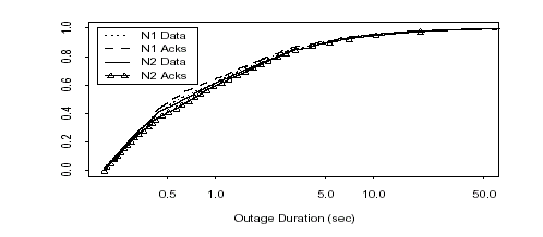
Figure : Distribution of packet loss outage durations exceeding 200 msec
Efficacy of TCP retransmission
Ideally, TCP retransmits if and only if the retransmitted data was indeed lost. However,the transmitting TCP lacks perfect information, and
consequently can retransmit unnecessarily.
Redundant retransmission (RR) means that the data sent had already arrived at the receiver, or was in flight and
would successfully arrive.
Three types of RRs:
unavoidable : because all of the acks for the data were lost;
coarse feedback : meaning that had earlier acks conveyed
finer information about sequence holes (such as provided
by SACK), then the retransmission could have
been avoided; and
bad RTO : meaning that had the TCP simply waited longer,
it would have received an ack for the data (bad retransmission timeout).
Ensuring standard-conformant RTO calculations and deploying the SACK option together eliminate virtually all of the avoidable redundant retransmissions. The remaining RRs are rare enough to not present serious performance problems.
Simulating how the global Internet data network behaves is an immensely challenging undertaking because of the network's great heterogeneity
and rapid change. The heterogeneity ranges from the individual links that carry the network's traffic, to the protocols that interoperate over the
links, to the "mix" of different applications used at a site and the levels of congestion (load) seen on different links.
Causes of Heterogenity
Topology : Constantly changing (dynamic routing),engineered by different entities
Links: Different types (slow and fast) ,asymmetric(satellite links)
Routes are asymmetric.
Protocol differences :Example Different TCP implementations.
Traffic generation:
Problem with trace driven solution : because of Adapative congestion control the trace intimately reflects the conditions at the time the connection occured.
Changes over time:
Also there is a limitation on the number of nodes a simulation can scale up to.
Coping Strategies
The search for invariants
The term invariant means some facet of Internet behavior which has been empirically
shown to hold in a very wide range of environments.
Some promising candidates:
1: Longer-term correlations in the packet arrivals seen in aggregated Internet traffic are well described
in terms of "self-similar" (fractal) processes.
2: Network user "session" arrivals are well described using Poisson processes.
3 :A good rule of thumb for a distributional family for describing connection sizes or durations is lognormal.
But these invariants are very difficult to find
Carefully exploring the parameter space
The basic approach is to hold all parameters (protocol specifics, how routers manage their queues and schedule packets for forwarding, network topologies and link properties, traffic mixes, congestion levels) fixed except for
one element,to gauge the sensitivity of the simulation scenario to the single changed variable. One rule of thumb is to consider orders of magnitude in parameter ranges (since many Internet properties are observed to span several orders of magnitude). In addition, because the Internet includes non-linear feedback mechanisms, and often subtle coupling between its different elements, sometimes even a slight change in a parameter can completely change numerical results.
Everything is measured at the 2 ends of the connection. The internet is considered as a black box.
How the properties are measured?
The properties are measured using tcp traces.
The advantages are :
1: The tcp traces are directly indicative of the TCP performance.This is because the TCP
traffic is "real world" as it is widely used in today's Internet.Consequently any network path
properties that we can derive from measurements of TCP transfer can potentially be directly applied to
tuning TCP performance.
2: TCP packet streams allow fine-scale probing without unduly loading the network,
since TCP adapts its transmission rate to current congestion levels.
The disadvantages are:
1: we need to distinguish between the apparently intertwined effects of the transport protocol
and the network.
2: TCP packets are sent over a wide range of time scales, from milliseconds to many seconds between
consecutive packets.Such irregular spacing greatly complicates correlational and frequency-domain analysis, because a stream of TCP packets does not give us a traditional time series of constant-rate observations to work with.
More on setup
This study of internet packet dynamics was conducted by tracing 20,000 TCP bulk transfers
between 35 Internet sites.
These sites run special measurement daemons i.e NPDs to facilitate measurement.With this framework the number of internet paths avaliable for measurement grows as N2(N square) for N sites yielding attractive scaling.
The first run N1 was conducted December 1994 and the second run N2 during Nov-Dec 1995.
The differences between N1 and N2 give an indication of how Internet Packet dyanamics changed during the course of 1995.
Each measurement was made by instructing daemons running at two of the sites to send or recieve a 100 Kbyte TCP bulk transfer and to trace the results using tcpdump.
Measurements occurred at Poisson intervals,which, in principle, results in unbiased measurement,
even if the sampling rate varies .
In N1 the the mean per-site sampling interval was about 2 hours, with each site randomly
paired with another.
In N2 sampling was done onpairs of sitres in a series of grouped measurements varying the sampling
rate from minutes to days, with most rates on the order of 4-30 minutes.
These groups then give observations of the path between the site pair over a wide range
of time scales.
Another difference between N1 and N2 was that in N2 Unox Sockets were used to assure that the sending and
the receiving Tcps had big windows to prevent window limitations from throttling the transfer's throughput.
The properties which measured were:
- Network pathologies such as reordering,replication and corruption
- Bottleneck bandwidth
- Packet loss
- One way delay
Packet reordering
Even though Internet routers employ FIFO queueing, any time a route changes, if the new route offers a lower delay
than the old one, then reordering can occur.
Detection of reordering
The reordered packets were recorded at both end of each TCP connection. Any Trace pairs suffering filter errors were removed.
Then for each arriving packet pi it is checked whether it was sent after the non-reordered packet.If so it becomes the new such packet .
Otherwise it's arrival is counted as an instance of network reordering.
Observations of reordering
There was significant amount of reordering. Overall there was 2% of all of the N1 data packets and 0.6% of the acks arrived out of order.
For N2 it was 0.3% of all data packets and 0.1% of acks. Thus the data packets were reordered more than the acks.
It was aslso observed that the out-of-order delivery varies from site to site .For e.g for the "ucol" site 15% of the data were reordered much higher
than the 2.0% average.
Also reordering was highly asymmetric. Only 1.5% of the data packets sent to ucol during N1 arrived out of order.
Thus, we should not interpret the prevalence of out-oforder delivery summarized above as giving representative
numbers for the Internet, but instead form the rule of thumb: Internet paths are sometimes subject to a high incidence of reordering, but the effect is strongly site-dependent, and apparently correlated with route fluttering, which makes sense since route fluttering provides a mechanism for frequently reordering packets.
Figure shows a sequence plot exhibiting a massive reordering event. This plot reflects packet arrivals at the TCP receiver, where each
square marks the upper sequence number of an arriving data packet. All packets were sent in increasing sequence order. Fitting a line to the
upper points yields a data rate of a little over 170 Kbyte/sec, which was indeed the true (T1) bottleneck rate ( 4). The slope of the packets
delivered late,though, is just under 1 Mbyte/sec, consistent with an Ethernet bottleneck. What has apparently happened is that a router with
Ethernet-limited connectivity to the receiver stopped forwarding packets for 110 msec just as sequence 72,705 arrived,most likely because at that point it processed a routing update. It finished between the arrival of 91,137 and 91,649, and began forwarding packets normally again at their
arrival rate, namely T1 speed. Meanwhile, it had queued 35 packets while processing the update, and these it now finally forwarded whenever it
had a chance, so they went out as quickly as possible, namely at Ethernet speed, but interspersed with newarrivals.
This pattern was observed a number of times not frequent enough to conclude it is anything but a pathology,but often enough to suggest that
significant momentary increases in networking delay can be due to effects different from both route changes and queuing most likely due to
forwarding lulls.
Effect of reordering
While out of order delivery can violate one's assumption about the network,the abstraction i.e well modelled as a series of FIFO queing servers
it was found that it had little impact on TCP performance.
The value of duplicate threshold Nd =3 was choosen primarily to assure the threshold e\was conservative.
Two possible ways to improve fast retransmit mechanism:
1:>By delaying the generation of dups to better idsambiguate packet loss from reordering and
2:>By altering threshold to improve the balance between seizing retransmission oportunities verses avoiding unneeded transmissions.
Packet reordering time scales:
The presence of spikes was found strongest at 81ms.
For N1 20ms would identify 70% of out of order deliveries.
For N2 8ms would identify 70% of out of order deliveries.
Thus a generally modest wait serves to disambiguate most sequence holes.
Degree to which false fast retransmit signals due to reordering are actually a problem.
Definitions
Rg:b : Ratio of good(necessary) to bad(unnecessary) reordering runs.
W : waiting time
For Nd = 3dups and W=0 N1 Rg:b =22 and N2 Rg:b =300.Clearly the current scheme works well.
While Nd=4 improves Rg:b by a factor of 2.5 it also diminishes fast retransmit opportunities by about 30% a siffgnificant loss.
For Nd=2 we gain 65-70% nore fast retransmit opportunities but Rg:b falls by factor of 3.
But if W=20ms Then Rg:b falls only slightly (30% for N1 and none for N2). But this requires both sender and reciever modifivations
increasing the problem of deploying the change.Thus safely lowering Nd is impractical.
Even usign Tcp SACK(selective acknowledgements)may help in some situations but it too poses above problems.
Packet replications
It was observed that packet replication rarely happened.It may happen at link level.
Packet corruption
Network delivers an imperfect copy of the original packet.
The proportion of Internet data packets corrupted in transit was found to to be around 1 in 5000.
The corruption was lesser in acks.
The corruption rate is not negligible as TCP uses 16 bit checksum because it means 1 in every
3 million packets are accepted with corruption i.e many packets a day.
If checksum were made to be 32 bits then only 1 in 2*10^13 packets would be accepted with corruption
Bottleneck Bandwidth
Difference between bottleneck bandwidth and available bandwidth:
Bottleneck bandwidth gives an upper bound on how fast can a connection possibly transmit data.
Available bandwidth denotes how fast a connection should transmit to preserve network stability.
Thus the former never exceeds the later and in fact can be much smaller.
For analysis the bottleneck bandwidth (Pb) is afundamental quantity because it
determines sel-inference time constant Qb which is the time required to forward a given packet
through the bottleneck element.
Qb = b/Pb
where b is number of bytes in a packet.
Packet pair is used for bottleneck estimation.The idea is that if 2 packets are transmitted by the sender with an interval Ts < Qb between
them,then when they arrive at the bottleneck they will spread out in time by the transmision delay of the first packet across the bottleneck:
after completing transmision through the bottleneck,their spacing will be exactly Qb.
If the measurements are made at the sender only then "ack compression" can significantly alter the spacing of the small ack packets as they return through the network distorting the bandwidth estimate
So reciever based packet pair is considered (RBPP) which is considerably more accurate than
source based packet pair (SBPP) since it eliminates additional noise and assymetry of the return path and also noise due to delay in generating acks themselves.
Sources of error
The main problems were
- out of order delivery
- Limitations due to clock resolutions of the reciever
- Changes in bottleneck bandwidth
- Multi-channel bottleneck links i.e channels which operate in parallel :here packets don't queue behind each other thus violating assumption of single end to end forwarding path leading to misleading over estimates
PACKET BUNCH MODES (PBM)
The main observation behind PBM is that we can deal with packet-pair's shortcomings by forming estimates
for a range of packet bunch sizes, and by allowing for multiple bottleneck values or apparent bottleneck values. By
considering different bunch sizes, we can accommodate limited receiver clock resolutions and the possibility of multiple channels or load-balancing across multiple links, while still avoiding the risk of underestimation due to noise diluting larger bunches, since we also consider small bunch sizes. By allowing for finding multiple bottleneck values, we again accommodate multi-channel (and multi-link) effects, and also the possibility of a bottleneck change.
It was found that RBPP with PBM performs significantly better than SBPP.Thus reciever support is required for good estimates.
PACKET LOSS
The packet loss was found to be 2.7% in N1 and 5.2% in N2.This is because of use of bigger windows in N2.
Ack loss give a clearer picture of the overall internet loss patterns while data loss tell us specifically about the conditions as percieved by the TCP
connections.
Network has 2 states quiescent (no ack loss observed) and busy.
How loss rates evolve over time.
Observing a zero-loss connection at a given point in time is quite a good predictor of observing zero-loss connections up to several hours in the
future, and remains a useful predictor, though not as strong, even for time scales of days and weeks . Similarly, observing a connection that
suffered loss is also a good predictor that future connections will suffer loss. The fact that prediction loses some power after a few hours supports
the notion developed above that network paths have two general states, quiescent and busy, and provides evidence that both states are long-lived,
on time scales of hours. The predictive power of observing a specific loss rate is much lower than presence of zero or non-zero loss. That is, even if
we know it is a busy or a quiescent period, the loss rate measured at a given time only somewhat helps us predict loss rates at times not very far
(minutes) in the future, and is of little help in predicting loss rates a number of hours in the future.
Data loss vs ack loss
Distinction was made betwen loaded and unloaded data
Loaded data packets : which had to queue at the bottleneck links
Unloaded data packets : which did not have to queue
Data loss rates was found more than ack loss.
Loss bursts
Packet loss was found to occur in bursts.
Successive packet losses were grouped into outages.
Figure : Distribution of packet loss outage durations exceeding 200 msec
Efficacy of TCP retransmission
Ideally, TCP retransmits if and only if the retransmitted data was indeed lost. However,the transmitting TCP lacks perfect information, and
consequently can retransmit unnecessarily.
Redundant retransmission (RR) means that the data sent had already arrived at the receiver, or was in flight and
would successfully arrive.
Three types of RRs:
unavoidable : because all of the acks for the data were lost;
coarse feedback : meaning that had earlier acks conveyed
finer information about sequence holes (such as provided
by SACK), then the retransmission could have
been avoided; and
bad RTO : meaning that had the TCP simply waited longer,
it would have received an ack for the data (bad retransmission timeout).
Ensuring standard-conformant RTO calculations and deploying the SACK option together eliminate virtually all of the avoidable redundant retransmissions. The remaining RRs are rare enough to not present serious performance problems.
SIMULATING THE INTERNET
Simulating how the global Internet data network behaves is an immensely challenging undertaking because of the network's great heterogeneity
and rapid change. The heterogeneity ranges from the individual links that carry the network's traffic, to the protocols that interoperate over the
links, to the "mix" of different applications used at a site and the levels of congestion (load) seen on different links.
Causes of Heterogenity
Topology : Constantly changing (dynamic routing),engineered by different entities
Links: Different types (slow and fast) ,asymmetric(satellite links)
Routes are asymmetric.
Protocol differences :Example Different TCP implementations.
Traffic generation:
Problem with trace driven solution : because of Adapative congestion control the trace intimately reflects the conditions at the time the connection occured.
Changes over time:
- New pricing structures
- New scheduling policies (Fair queuing)
- Native multicast becomes widey deployed
- Mechanisms for supporting different classes of service
- Web caching becomes ubiquitous
- A new bandwidth hungry killer application (multi player gaming) comes along.
Also there is a limitation on the number of nodes a simulation can scale up to.
Coping Strategies
The search for invariants
The term invariant means some facet of Internet behavior which has been empirically
shown to hold in a very wide range of environments.
Some promising candidates:
1: Longer-term correlations in the packet arrivals seen in aggregated Internet traffic are well described
in terms of "self-similar" (fractal) processes.
2: Network user "session" arrivals are well described using Poisson processes.
3 :A good rule of thumb for a distributional family for describing connection sizes or durations is lognormal.
But these invariants are very difficult to find
Carefully exploring the parameter space
The basic approach is to hold all parameters (protocol specifics, how routers manage their queues and schedule packets for forwarding, network topologies and link properties, traffic mixes, congestion levels) fixed except for
one element,to gauge the sensitivity of the simulation scenario to the single changed variable. One rule of thumb is to consider orders of magnitude in parameter ranges (since many Internet properties are observed to span several orders of magnitude). In addition, because the Internet includes non-linear feedback mechanisms, and often subtle coupling between its different elements, sometimes even a slight change in a parameter can completely change numerical results.