APPROXIMATE CELL DECOMPOSITION

APPROXIMATE CELL DECOMPOSITION

INTRODUCTION :-

· This approach has a basic difference with exact cell decomposition approach. Here the cells have a pre-specified shapes, which are generally rectangloid.

· Because of this prespecification of shapes of cells we are not able to represent the free space exactly.

· Thus the name approximate cell decomposition.

· And as in the exact cell decomposition approach, a connectivity graph is found out representing the adjacency relation among the cells and a path is searched.

GENERAL DESCRIPTION :-

· A Rectangloid represents a closed region of the following form in a Cartesian space Rⁿ :

{(x₁,x₂,…..,x_n) / x₁Є [x₁^’,x₁^’’], …. , x_nЄ [x_n^’,x_n^’’]} .

The differences x_i^’’ – x_i^’ , for i = 1, 2, … , n are called the dimensions of the rectangloid. And none of these dimensions can be zero.

· CB represents the C-obstacle region, and D represents the rectangloid. Let R represents the space inside D. i.e. R = int(D).

Then C_free= R \ CB.

· A rectangloid decomposition P of Ω is a finite collection of rectangloids {κ_i}_i=1,2,..,r such that :

- Ω is equal to the union of κ_i i.e. :

Ω = union of(κ_i)

- The interior of κ_i’s do not intersect, i.e. :

For all i₁, i₂ Є [1,r] i₁ ≠ i₂ : int(ki₁) ∩ int(k_i2) = φ.

Each rectangloid k_i is called a cell of the decomposition P of Ω.

· A cell is classified as :

- EMPTY, if and only if the interior does not intersect with the C-obstacle region, i.e. int(k_i) ∩ CB = φ

- FULL, if and only if, k_i is entirely contained in the C-obstable region.

- MIXED, if a cell is neither empty nor it is full it is mixed.

· Two cells are called adjacent if and only if their intersection is a set of non-zero measure in R^m-1.

· The connectivity graph of the decomposition P of Ω is a non directed graph G, whose nodes are the EMPTY and the MIXED cells of P and the nodes of connected by a link if and only if the corresponding cells are adjacent.

· Given a rectangloid decomposition P of Ω a path is defined as a sequence (k_ji)_i=1,2,…p of EMPTY or MIXED cells such that any two consecutive cells in this sequence are adjacent cells.

· A path that only contains EMPTY cells is called an E – path.

· A path that contains at least one MIXED cell is called a M – path.

HOW TO FIND A FREE PATH :-

Given the initial configuration of the robot q_initand the final configuration of the robot q_goal both belonging to the C_free if we can find out an E – path (k_ji)_i=1,…,p such that q_initЄ k_j1 and q_goal Є k_jp a free path can be found out which joins the initial to the goal configuration using the E – path linking q_init to q_goal by a polygonal line whose vertices are the points Q_j which belong to the face which is common between each of the two adjacent cells of the E – path.

Or in other words,

Q_j Є int(B_j), where B_j = boundary(k_ji) ∩ boundary(k_j(i+1)) , j= 1,… p-1

THE BASIC ALGORITHM :-

1. Compute a rectangloid decomposition P₁ of Ω. Set it to 1.

2. Search the connectivity graph G_i associated with the decomposition P_i for a channel connecting the initial cell containing q_initto the goal cell containing q_goal . If the outcome is an E – path return success. If the outcome is an M – path goto 3. Otherwise return failure.

3. Let M_i be the M – path generated at step 2. Set P_i+1 to P_i .For every MIXED cell k in M_i compute a rectangloid decomposition P^k for k and set P_i+1to [P_i+1\{k}] U P^k. Increment i by 1. Go to step 2.

HOW WE ACTUALLY GO AROUND COMPUTING A RECTANGLOID DECOMPOSITION?

THE METHOD OF DIVIDE AND LABEL :-

· First we divide the cells into smaller cells of equal dimension.

· And then we lebel the newly created cells according to their intersection with the C-obstacle region as EMPTY, FULL, or MIXED.

· This is the basic computation in step 1 and step 3 of the algorithm proposed above.

2^m– Tree Decomposition :-

· This is the most widely used method to decompose a rectangloid where m is the dimension of the configuration space.

· A 2^m tree decomposition of Ω is a tree of degree 2^m (each node has 2^m children).

· The root of the tree is Ω itself.

· All nodes have 2^m children and each are either labeled EMPTY or FULL or MIXED.

· Only nodes which are of MIXED types have children.

· The decomposition is done such that all the children are of equal dimensions.

· If m = 2 the tree is called a quadtree. If m = 3 the tree is called an octree.

· The depth of a node determines the dimension of the corresponding cell relative to Ω.

· The height h of the tree determines the resolution of the decomposition of Ω.Which gives the size of the smallest cell present in the decomposition tree.

· For the algorithm we need to specify the initial height h₁ of the decomposition tree. And all the MIXED cells which are at the depths less than h₁ are decomposed at this step.

· An maximal height h_max og the tree is also specified in order to bound the iterative process carried out by steps 2 and 3. Every mixed cell whose depth is equal to h_max is re-lebeled as FULL.

· In the worst case the number of leaves in a 2^m decomposition tree of height h will be 2^mh. Hence it increases exponentially with dimension of C and the depth of the decomposition.

· Though practically the number is not so large as the tree is pruned at every EMPTY or FULL node.

CELL LEBELLING IN R^N:-

· Assumed that the robot and the obstacles are both of polygonal type and only the robot is allowed to translate or we describe the C-obstacle region by the disjunctive expression called a C – sentence :

V Λ e_ij

ⁱ ^j

where e_ij is a C – constraint of the form a_ijx + b_ijy + c_ij <= 0. Here each conjunct

Λ e_ij represents the C – obstacle of one polygonal obstacle.

· A C–sentence S_k is associated with every MIXED cell k.

· A cell k is said to be inside the C-constrint e_ij if all the points (x,y) Є k satisfy e_ij. In other words :- if each of its vertices verifies : a_ij x + b_ij y + c_ij < = 0

· A cell k is said to be outside the C-constraint e_ij if all the points (x,y) Є k contradict e_ij .In other words :- if each of its vertices verifies : a_ij x + b_ij y + c_ij >= 0

· A cell k is said to be cut by the C-constraint e_ij if the cell is neither inside nor outside e_ij .

ALGORITHM FOR LEBELLING OF NEW CELLS :-

· Let S is the C-sentence associated with the parent cell of k.

Function LABEL(k, S) {

For each conjunct Λ e_ij Є S do {

For each C-constraint e Є Λ e_ij do {

If k is inside e then

Λ e_ij = Λ e_ij \ {e}

Else if k is outside e then

S = S \ { Λ e_ij}

}

if Λ e_ij Є S and Λ e_ij =φ then {

label k with FULL;

exit(0);

}

if S = φ then {

label k with EMPTY;

}

else {

label k with MIXED;

associate S with k;

}

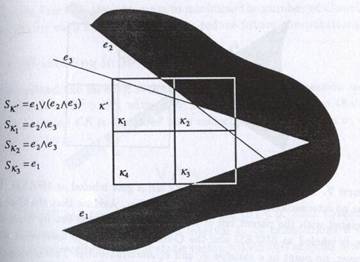
Fig (1) from the book textbook robot motion planning , describing the labeling technique as discussed in the algorithm.

This procedure takes O(n) time to label a cell where n is the number of C-constraints in the input S.

· In this procedure we see a new simplified S is associated with newly labeled MIXED cells. This considerably decreases the computation time for the labeling of forthcoming cells.

· Since each C-constraints is treated independently while labeling sometimes cells may get labeled MIXED even though they are not. It may happen when a cell k is not outside the C-constraints e₁ and e₂although no point of the cell k is inside both e₁ and e_2. however this will no lead to an error as on the next iteration when that mixed cell will be decomposed each of the cells will be labeled correctly as EMPTY.

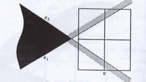
Fig (2) from the textbook robot motion planning, which shows the case of conservation described above.

HOW WE GO ABOUT SEARCHING THE CONNECTIVITY GRAPH?

HIERARCHIAL GRAPH SEARCHING :-

· This algorithm constructs a hierarchy of CG’s . The CG at the root corresponds to the first decomposition P₁ of Ω . Let us denote the connectivity graph for the cell k as G^k.

· The graph G^Ω is searched for a path connecting q_init to q_goal .

· If an M-path M₁ is found every MIXED cell in M₁ is decomposed and searched for a path that connects q_init to q_goal that connects appropriately to the rest of the M₁.

· If an E-path is found out then we are done. Else if we cannot find out an E-path then we return a failure.

THE ALGORITHM :-

1. Find out the path M₁ using CG G ^Ω . If M₁ is an E-path. We are done.

2. If M₁ is an M-path we construct another path M₂ as follows :

We go on considering every successive cell k in M₁ starting with the cell that consists of q_init. If k is empty it is added to the new path M₂ else if its MIXED , it is decomposed into a set P^k of smaller cells. Let G^k be the CG associated with P^k .G^k is then searched for a path M^k which satisfies the following conditions.

1. If the cell k is the first cell in M₁ then the first cell in M^k must contain q_init.

2. If the cell k is the last cell in M₁ then the last cell in M^k must contain q_goal .

3. If k is not the first cell in M₁ then the first cell of M^k must be adjacent to the last cell of the current M₂ .

4. IF k is not the last cell in M₁ then the last cell of M^k must be adjacent to the subsequent cell in the current path M₁.

3. This M^k is appended to M₂ and we carry on the procedure presented in step 2 until we exhaust all the cells of M₁ .

4. If the new path is an E-path, we can find out a polygonal path using M₂. else we set M₁ to M₂ and go to step 2.

· It may be possible that we could not find out a free-path even after we decompose the C-space to the maximum resolution. In such case we return a failure.

Submitted by :-

VIVEK VAIBHAV

Email id – vivekv@cse.iitk.ac.in

Λ eij represents the C – obstacle of one polygonal obstacle.

Λ e_ij represents the C – obstacle of one polygonal obstacle.