1. Introduction

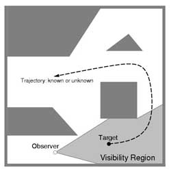
Figure 1. The goal is to maintain visibility of a moving target that may or may not be predictable.

Several applications require persistent monitoring of  a moving target by a controllable vision system. The applications include mobile robotics and automated processes. A motion planning problem is considered here in which a robot carries a camera that must maintain visibility of a target in a cluttered workspace. The primary distinction between the problem considered and standard tracking problems is the introduction of global, geometric constraints on both visibility and robot configurations. The following conditions are assumed:

    1) an observer must maintain visibility of a moving target;

    2) the workspace contains static obstacles that prohibit certain configurations of both the observer and target;

    3) the workspace also contains static obstacles that occlude the target from the observer;

    4) a (possibly partial) motion model is known for the target.

The first condition implies that target tracking is the primary interest, and visibility can be defined in a variety of ways, depending on the particular problem. The second condition introduces the geometric constraints that appear in the standard path planning problem. The third condition complicates the tracking problem by prohibiting pairs of observer and target configurations at which the observer cannot ``see'' the target. In many cases an obstacle in the workspace will cause both motion and visibility constraints. The fourth condition provides predictive information that should be utilized when designing a strategy. For example, the entire trajectory of the target might be known, or alternatively, only a velocity bound might be known. In addition to the previous four conditions, it might also be important to optimize some criteria such as the total distance traveled, energy utilized by the observer, or the quality of the visual information. This quality of visual information will be the aesthetic appeal of the final image, wherein cinematographic principles will be used as the optimizing variables.
 
 

2. Problem Formulation

Suppose that an observer and a target exist in a bounded, Euclidean workspace that is cluttered with static obstacles. Let C^o_free and C^t_free denote the free configuration spaces of the observer and target, respectively. Let X = C^o_free X C^t_free represent the state space. Let the index k refer to the stage or time step that occurs at time (k-1)Δt for some fixed Δt.

The observer will be controlled through actions, u_k , chosen from some action space U . The discrete time trajectory will be given by a transition equation of the form q^o_k+1 = f^o(q^o_k , u_k ), which yields a new configuration of the observer for a given current configuration and action.

The target will be described by a similar transition equation; however, the actions that control the target are generally unknown to the observer. Let  q^t_k+1  =  f^t(q^t_k , θ_k) , in which θ_k represents unknown actions, chosen from some space Θ. One important special case,
which is the subject of Section 3, is when the target is predictable. In this case the transition equation can be represented as q^t_k+1  =  f^t(q^t_k). Together, f^o and f^t define a state transition equation of the form x_k+1 = f(x_k , u_k , θ_k).

Let X₀ is a subset of  X represent the visibility subspace, which corresponds to the set of all states for which the visibility relation holds.
 

Next consider evaluating a state trajectory. Abstractly, the goal is to control the observer to ensure that the state remains in X₀. The cost of applying a sequence of control inputs is state trajectory can be expressed as

                L(x₁,......,x_K,u₁,.......,u_K) = Σ l_k( x_k,u_k) + L_K+1(x_K+1)                                      ( 1 )

in which K represents the final time increment for issuing a action and l_k( x_k,u_k) is a loss that accumulates in a single time step. The final state, x_K+1 can also be penalized, using L_K+1 . A simple, useful form of  l_k is

                 l_k( x_k,u_k) = { 0 if x_k belongs to  X₀ ; 1 otherwise }                             (2)

This loss functional measures the amount of time that the target is not visible. One could also include a cost for choosing actions that produce motion. This would allow the robot motions to be optimized in addition to the time that the target is in view. The loss functional evaluates a given trajectory.

3. Predictable Targets

In this section the assumption is made that q^t_k is known for all k belonging to {1,.....,K+1}. In this case, the state transition equation reduces to q_k+1 = f(x_k,u_k), which implies that the state trajectory, {x₂,.......,x_K+1} is known once x₁ and inputs {x₁,.......,u_K+1} are given.

For a problem that does not involve optimizing the robot trajectory, motions for the observer could be determined by recursively computing visibility and reachability sets from stage K+1 down to stage 1. Suppose the target and observer are both points. Let V_k denote the subset of the free space from which the target is visible. Let A_k1 denote the set of all locations from which the
observer could move at stage k -1 and lie in V_k at stage k. At any stage the observer must lie in the intersection of the two sets V_k and  V_k. A feasible trajectory for the observer can be obtained by back chaining from the final stage, guaranteeing accessibility and visibility in each step, until a set of possible initial states is obtained.

3.1 Computational Approach

The computational approach can be organized into four basic steps:
1. Construct a discretized representation of  C^o_free, in which K = {1,.....K+1}.

2. For each k, mark all discretized values of q^o_k from which the target (at known q^t_k ) is visible.
3. Within X₀ for each stage from K + 1 to 1 perform dynamic programming computations with interpolation.
4. Extract the optimal sequence, {u*₁,........,u*_K}, using cost­to­go representations.

For the sample solutions below the target moves at its maximum speed of 3 units/stage. The observer is controlled through the simple holonomic model,

                        q^o_k+1 = q^o_k + u¹_k Δt[ cos(u²_k ) sin(u²_k ) ]^T          (3)

in which u¹_k ≥ 0 represents the speed of the observer, and u²_k ε [0, 2π) represents the direction of motion. No dynamics are considered in this model.

Figure 2 shows a simulation of a trajectory that is obtained from the computed optimal strategy. The actions u¹_k = 0 (no motion) and u¹_k = 3 and u²_k ε [0, 2π) (motion at a fixed speed in some direction) were allowed. The loss functional is of the form l_k( x_k,u_k) = l_m + l_v . The term l_m is a penalty for motion, and l_m = 0 if u¹_k = 0, otherwise l_m = 1. The term l_v is a penalty for losing visibility, which is much more important, yielding l_v = 500. There are 105 stages for this problem, and the dynamic programming computations took about 20 seconds on a SPARC 20 workstation. Note that although the target trajectory is quite long, the distance traveled by the observer is short. An initial position for the observer was automatically selected from which the target was visible during the first portion of the trajectory. 

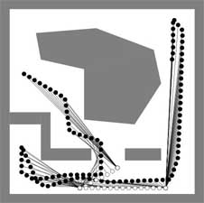
Figure 2. A simulation is shown of the optimal state trajectory for a tracking problem. The observer strategy, including the initial position, is chosen to maintain visibility and minimize the total distance traveled. The target positions are shown as black circles, and the target trajectory starts in the upper left. The observer positions are shown with white circles. The line of sight is shown between the observer and target at each stage.

The example in Figure 3a involves the same geometry; however, the loss functional is slightly changed to yield l_v = 0 only if the target is both visible and the distance between the target and observer lies within 10 and 25 units. Also, the speed, u¹_k , is allowed to vary
between 0 and 3, with a loss, l_m , that is proportional to the speed. In this case, the observer must travel a greater total distance, yet an optimized trajectory that maintains visibility is still obtained. Figure 3b shows an example in which the maximum observer speed is 1.5, and the target speed is 3.0. There are many visual obstructions, and the observer is able to maintain visibility of the target in all but two stages. During this period, the observer moves quickly to the right to reacquire the target. 

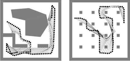
Figure 3. a) This example differs from the previous one by additionally requiring that the observer remains within a specified distance range from the target; b) In this example, the target can moves at twice the maximum speed of the observer. In the optimal trajectory of the observer, there are only two stages in which the target is not visible.

Bibliography:

1.   Motion Strategies for Maintaining Visibility of a Moving Target. by Latombe et. al.