POTENTIAL FIELD METHODS
Motivation
The potential field approach to motion generation
consists of regarding the robot in configuration space as a unit mass particle
moving under the influence of the force field F = -(gradient) U. This method
is well suited when the obstacle are not known in advance, but are sensed
during motion execution. Different techniques have been developed for path
generation using the potential field. The depth-first technique may get
stuck at local minima of the potential function. The second technique operates
in a best-first mode. It deals with the local minima by filling them
up. However, when the dimension, m of the configuration space becomes large,
filling up local minimum wells is no longer tractable. On the other hand,
the construction of a navigation function, i.e. a potential field with
no local minimum other than the goal configuration, is a difficult problem
that has a known solution only when the C-obstacles have simple shapes
and/or when the dimension of the configuration space is small (m = 2 or
3). To overcome the abovementioned limitations, Randomized Path Planner
(RPP) was proposed.
We describe the two techniques : Best-first planning, Randomized
motion planning.
Best First Planning
Given a configuration
q in the m-dimensional grid
GC, its
p-neighbors (1<= p <= m) are defined as all the configurations
in GC having atmost p coordinates differing from those of
q, the amount
of the difference being exactly one increment in absolute value.
procedure BFP;
begin
install qinit in T; [initially
T is the empty tree]
INSERT (qinit, OPEN); mark qinit
visited;
[initially, all the configurations in GC are marked
unvisited]
SUCCESS <- false;
while ¬ EMPTY(OPEN) and ¬ SUCCESS do
begin
q
<- FIRST(OPEN);
for every neighbor q' of q in GC do
if U(q') < M and q' is not visited then
begin
install q' in T with a pointer toward q;
INSERT(q', OPEN); mark q' visited;
if q' = qgoal then SUCCESS <- true;
end;
end;
if SUCCESS then
return the constructed path
by tracing the pointers in T
from qgoal
back to qinit;
else return false;
end;
The algorithm is guaranteed to return a free path whenever there exists
one in the free subset of the grid GC and to failure otherwise.
The size of GC is O(rm) where r is the number of discretization
points along each coordinate axis.
If we represent OPEN as a balanced tree, INSERT and FIRST takes logarithmic
time in size of OPEN which can be O(rm) in the worst case. The
time complexity of the algorithm is thus O(mrm log r).
Randomized motion planning
Overview
We assume that the potential function, U>=0 and
that any configuration q such that U(q) = 0 is a goal configuration.
The RPP constructs and searches a graph G whose nodes are local minima
of the potential function U. Two minima are connected by a link in the
graph if the planner has constructed a path joining them.
The planner starts at the input initial configuration
qinit.
From there, it executes a best-first motion, i.e. it follows the
steepest descent of the potential U. The best-first motion stops when it
reaches a minimum
qloc. If U(qloc)
=0, the problem is solved and the algorithm returns the constructed path.
Otherwise, it attempts to escape from the local minimum by executing a
series of
random motions
issued from
qloc. Each
random motion is immediately followed by a new best-first motion that attains
a minimum. If this minimum is different from qloc, it
is installed as a successor of qloc in the graph G. Hence, two
adjacent minima in G are connected by a path obtained by composing a random
motion and a best-first motion. We proceed like this till the goal configuration
is attained or the planner gives up.
Best first motion
The potential U may not tend to infinity when the
robot's configuration gets closer to the C-obstacle region. Hence a best-first
motion is not collision free. The planner must verify that the next chosen
configuration qi+1 lies in the free space. When m is
small, best-first motions can be generated by using the m-neighborhood
in GC. However, when m becomes larger, it is too large to be explored at
every step. One way to take care of this is to check only a small number
of randomly selected m-neighbors. If none is selected, we consider qloc
to be local minimum.
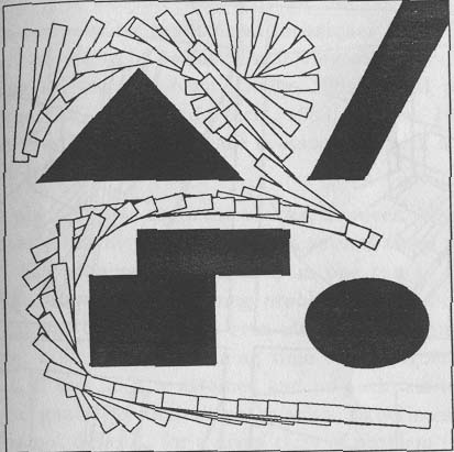
Random motion
Random walks:
A series of t motion steps such
that the projection of every step along each axis x
i, i = 1, 2, ..., m is
randomly DELTA
i or -DELTA
i.
Random motions are executed whenever a local minimum
qloc
is encountered. Let us assume that each step takes a unit of time, so
that t is the duration of the random walk. Without the loss of generalization,
let us take the local minimum
qloc as the coordinates'
origin. The configuration after the random walk will be Q(t) = ( Q
1(t),Q
2(t), ..., Q
m(t) )
which verifies the following properties :
-
The density of Qi(t) is :
-
The standard deviation of Qi(t) is :
The planner should check for collision during the random path. If the new
configuration is not free, the planner randomly selects another candidate
configuration.
What should be the value of t ?
Should neither be too small nor too large.
Attraction radius Ri(qloc ):
the distance along the xi-axis between qloc
and the nearest saddle point of U in that direction.
The minimum distance that the robot must travel along any xi-axis in
order to escape from the local minimum is precisely Ri(qloc
).
Therefore, t could be defined as :
Graph Searching
- Iteratively generating successors of the local minimum (under consideration)
having the minimum potential value and limiting the number of random motions to
a predefined value K.
Drawbacks :
- Same local minimum may be attained several times.
- This may also waste time exploring a local minimum well containing smaller
local-minimum well imbricated in one another.
- If U(q'loc ) > U(qloc ), we ignore q'loc
; otherwise it generates its successors in the same fashion. (Note : If goal
configuration is encountered, the problem is solved ). If no local minimum with
potential value less than qloc is attained, it is considered
to be a dead-end and the search is resumed at the most recently considered local
minimum whose K successors have not been generated yet.
Drawbacks:
- If a low local minimum is attained, the planner may have difficulty
attaining a lower one from it.
- In this approach, instead of memorizing the whole graph we
proceed by remembering only the constructed path t connecting
the initial configuration to the current configuration. The planner iteratively
generates K random motions. If a lower local minimum q'loc is
attained then the planner appends the path from qloc to q'loc
to the path t and proceeds from q'loc
in the similar fashion. However, if no such q'loc is
attained, the planner randomly chooses a configuration qback
in the subset of t formed by random motions, and
backtracks to qback .
procedure RPP;
begin
t <- BEST-FIRST-PATH (qinit
); qloc <- LAST(t);
while qloc != qgoal
do
begin
ESCAPE <-
false;
for i
= 1 to K until ESCAPE do
begin
t <- RANDOM-TIME;
t <- RANDOM-PATH (qloc , t0);
qrand <- LAST (ti);
ti <- PRODUCT (ti
, BEST-FIRST-PATH (qrand));
q'loc <- LAST (ti);
if U(q'loc ) < U(qloc ) then
begin
ESCAPE <- true;
t <- PRODUCT (t ,
ti);
end;
end;
if ¬
ESCAPE then
begin
t <- BACKTRACK (t,
t1, ..., tK);
qback <- LAST (t);
t <- PRODUCT (t ,
BEST-FIRST-PATH (qback));
end;
qloc
<- LAST (t);
end;
end;
Path Smoothing
Iteratively replace subpaths of decreasing lengths with straight line
segments in the space Rm containing the grid GC. The segments are inserted in
the top-down order of the length going down to the grid resolution. Collision
checking has to be done at every insertion. More sofisticated variational
calculus techniques may be applied to optimize more involved objective criteria.
References
[1]. Robot motion planning , Jean Claude Latombe, Kluwer Academic publishers.
[2]. Barraquand, J. and Latombe, J.C., "A Monte-Carlo Algorithm for Path
Planning with Many degrees of freedom", Proceedings of the IEEE
International Conference of Robotics and Automation, Cincinnati, OH,
1712-1717
Submitted by :
Vidit Jain (98395)
(@iitk
or @yahoo)