A microscopic theory of traffic flow, i.e.,a theory of traffic flow which can predict the action of individual drivers over time in different driving situations, is an important and essential aspect of the area of traffic science and engineering. Since the early 1990s, microscopic simulation models have emerged as important tools for intelligent transportation system strategies.As basic and important components of a microscopic traffic simulation model, the car-following models has received considerable research interest.
Traditionally, traffic models have been developed using fluid flow analogies. This assumes that a highway can be represented by a link that has a certain flow capacity. This may be acceptable when traffic flows freely but this model modelling approach breaks down under congested traffic conditions.
Microscopic models differ from traditional computational models in that they
have significant random components and attempt to represent the dynamic nature
of traffic systems by simulating the interactions of individual vehicles. They
model numerous components of traffic flow and their influences, and therefore
provide more accurate traffic flow information, which is necessary for the
analysis of congested road networks.
Microsimulation models also differ in that vehicles move in the system in
real-time and are modelled according to the behaviour of vehicle drivers.
Researchers have indicated that vehicle drivers perform according to their
aggression and awareness.In traffic engineering terms this can be accounted for
in terms of simple rules of car-following, gap acceptance and vehicle
kinematics.
These models can be developed using various approaches viz fuzzy inference based
approach, multiregime approach etc.In the following work, a structure based on
the potential field theory of robot motion planning which can be used to model
driver behaviour in variety of driving situations is being discussed.
Traditionally driver behaviour has been modelled differently for different driving scenarios. For example there is a model for car-following behaviour, a model for lateral displacement etc.A single model structure that can predict driver behaviour in various driving situations will be discussed.
The driver's behaviour at all times, it is assumed, is
motivated by his concern for safety and his urge to minimize the travel time. Further
it is assumed that the driver views his travelling environment as a
conglomeration of obstacles which need be to be avoided in order to proceed
safely.
Sometimes the driver may choose a point on the road as a goal point which he
would like to reach while driving in this environment of obstacles. Such an
understanding of the driving allows the development of a single model structure
because all features such as road-edge, pot-hole, lane marking, other vehicles
on the road, etc can be viewed as obstacles albeit with different properties.
The model being discussed will be able to predict the driver's (or the test
vehicle's ) action in terms of choice of steering angle and acceleration or
deceleration , given a driving scenario. First the principles on which the model
is based will be discussed followed by the description of the model to predict
the position of the test vehicle on the road and the velocity of test vehicle
over time.
1.) The driving environment is characterized by the presence of
obstacles , either static or dynamic, and in certain cases the presence of
an
immediate goal.
2.) Each obstacle emanates some potential (or force ) around it; the
potential (or force) field of an obstacle is repulsive in nature. A goal
also
emanates a potential field , which however is
attractive in nature.
3.) The potential field emanated by an obstacle depends on the
properties of the obstacle. For example, the potential field due to a parked
vehicle may be assumed to be more prominent than
the potential field due to a small pothole.
4.) The potential at any point on the road is the algebraic sum
of all the potentials due to the driving environment features (i.e.,obstacles
and
goal) around that time.
5.) The test vehicle is assumed to move from one cross section of the road to the next. These cross-sections can be arbitrarily close.
6.) While moving from one cross section to the next, the driver of the
test vehicle always chooses a point with smallest potential among all
the
accessible points depend on the test vehicles
present orientation and the maximum steering angle.
7.) There exists an inverse relation between velocity at a point and
the potential at that point. The velocity corresponding to the potential
at a
point is referred to as the sustainable velocity. For
example, the speed on a narrow empty road is generally lower than the speed on a
broad empty road.
8.) The response of the test vehicle at a given point in terms of
acceleration or deceleration (referred to as longitudinal response as opposed to
lateral response) is a function of the rate
of change of potential ( faced by the driver) as well as the difference between
the current velocity
of the test vehicle and the sustainable
velocity at that point.
A model of driver behaviour is developed based on the principles presented above.
Let (x,y) represent the Cartesian space in which the road as well as all its features are defined; let Ui(x,y) be the potential field emanated by obstacle i;and let U(x,y) be the potential at the point (x,y) on the road;
Then based on principle 4, the potential at any point (x,y) is calculated as U(x,y) = Si Ui(x,y)
The term "position profile" refers to the path of of TV on the road over time as predicted by the proposed model. In general, the position profile is described graphically with distance from the left edge of the road as the abscissa and distance along the road as ordinate.
Position profile as suggested in principle 6 , is affected not only by the potential at different road points but also by the constraint of the maximum steering angle. This latter constraint restricts the number of points which the TV can access from its present location.
If ( xn,yn) represents the coordinates of the nth
cross section and (xna,yna) represents the
coordinates of the accessible points in the nth cross section then as per
principle 6 , the position of the TV (xn*,yn*) , at the nth
cross section is obtained such that
U (xn*,yn*) = min U(xn,yn)
,
(xn,yn) € An
where An represents the set of all accessible points in the nth cross section.
The set An can be determined from the current orientation of the TV and the maximum steering angle restrictions.
The " velocity profile" refers to the predicted velocity of TV along the position profile. The predicted velocity is obtained from the acceleration or decelerations (longitudinal response) of the TV at every instant of time . The acceleration/ deceleration is obtained using the longitudinal response model developed on the basis of principle 8.
If a(t + T) is the response of the TV at time t + T then as per Principle
8:
a(t+ T)
= f (U'(x*,y*) ,Vs(t) , Va(t))
where , T is the reaction time of driver , (x*,y*) is the position of the vehicle at time t , U'(x*,y*) is the rate of change of potential faced by TV at time t, Va(t)is teh actual velocity of TV at time t, Vs(t) is the sustainable velocity of teh TV at time t.The sustainable velocity is an inverse function of U(x*,y*) ; i.e., Vs(t) = g(U(x*,y*) ). In this work the functional form used is Vs(t) = c1-c2 U(x*,y*) where c1 and c2 are positive constants.
Functional form for longitudinal response model
As stated earlier, the model views the driving environment as a set of obstacles and immediate goals (jointly referred as features) . Further, the model also assumes that these features emit a potential field and that drivers react to the potential they face while travelling.
Goals are assumed to be of a single kind which basically states the preferred location of the driver of TV. However ,obstacles can be of various kinds. The two broad classes of obstacles are: (i) static obstacles (ii) dynamic obstacles . Static obstacles include features like road edges, pot-holes, lane marking , parked vehicle etc. whereas dynamic obstacles are primarily of two types : (i) vehicle moving in the direction of TV (referred to as same direction vehicle, SDV) (ii) vehicles moving in the opposite direction of TV ( referred to as opposite direction vehicles , ODV) .
In the following discussion potential field functions for dynamic obstacles and goals only would be presented
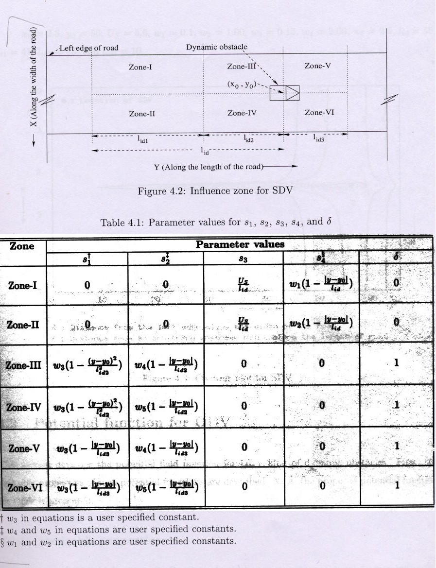
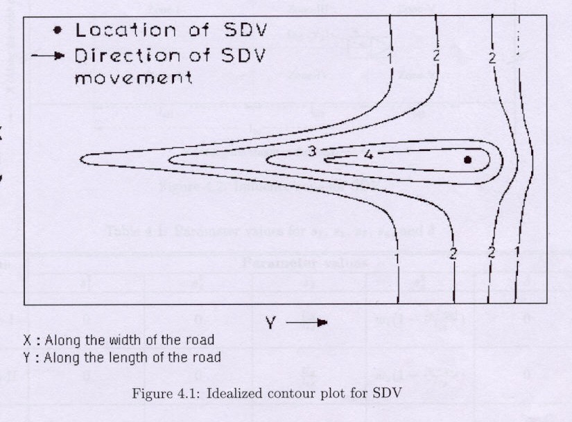
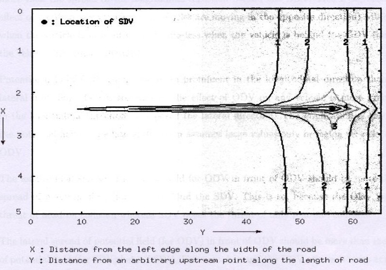
1.) The potential field function at all points should be greater than or equal to zero indicating repulsion.
2.) The potential function should be continuous and should decrease monotonically as one moves away from the SDV.
3.) The spread of the potential field in the longitudinal direction behind the SDV is more than that ahead of the SDV.
4.) Potential field should be more prominent in the longitudinal direction than in the lateral direction. The implication of this is that the field in the lateral direction assumes large values only in a direction very close to the SDV.
max [0, h(x,y)]
(x,y) lies in any zone
USDV =
min [h(x,y), h1(y)]
h(x,y) >= 0 and (x,y) lies in Zone-III , Zone-IV
min [h(x,y), h2(y)]
h(x,y) >= 0 and (x,y) lies in Zone-V , Zone-VI
where,
h(x,y)
= [ s1/|x -x0| + s2]d
+ [s3 (lid - | y - y0|)(1- |x -x0|
/s4)](1-d
)
h1(y)
= US [1 - |y -y0|/(lid1 + lid2) ]
h2(y) = US (1 - |y -y0|/ lid3
)
where, (x0,y0 ) are the co-ordinates of SDV, US
is the potential at (x0,y0 ) , lid1 , lid2
and lid3 are the distances from the SDV in the y-direction.
In the above equation values of s1, s2 , s3 ,
and d
depend on the co-ordinate of points (x,y) and the zone in which (x,y) lies on
the road.
The above function although complex in its algebraic description , produces a potential field function similar to the one described before
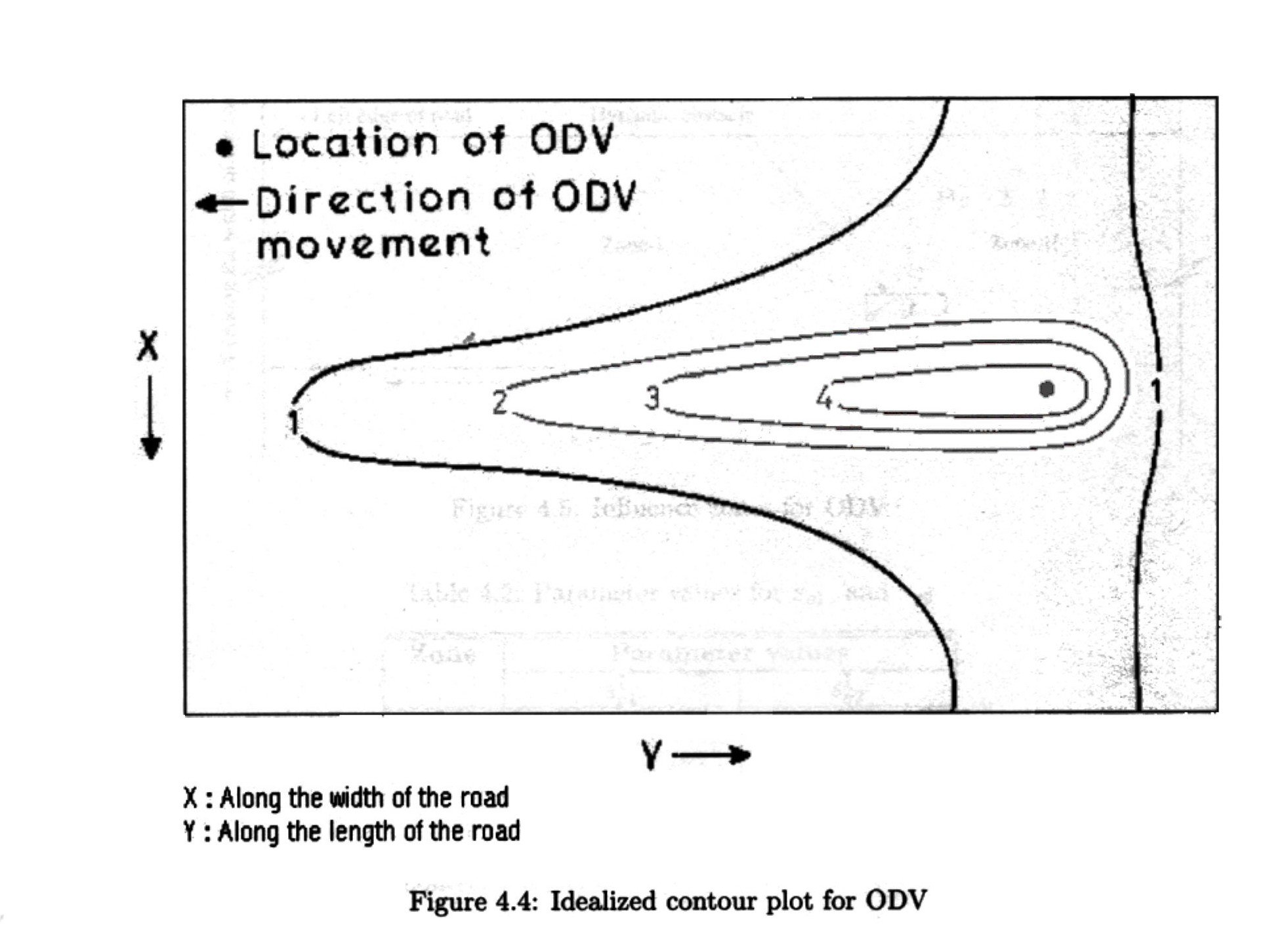
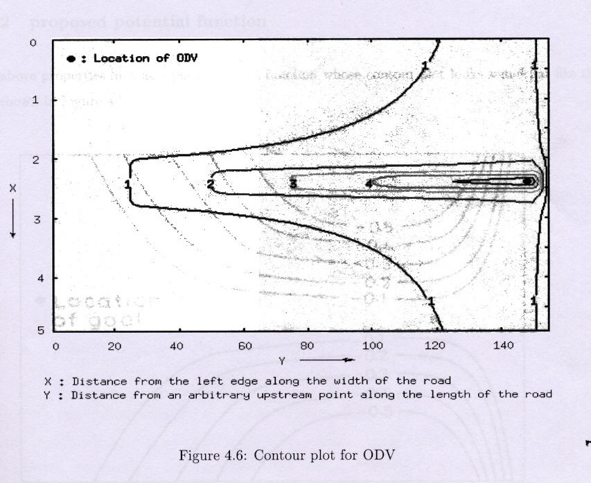
1.) The potential field function at all points should be greater than or equal to zero indicating repulsion.
2.) The potential function should be continuous and should decrease monotonically as one goes away from the ODV.
3.) The spread of the potential field in the longitudinal direction ahead of the ODV is more than that behind the ODV.
4.) Potential field should be more prominent in the longitudinal direction
than in the lateral direction. The implication of this is that the field
in the lateral direction assumes large values only in a
direction very close to the ODV.
5.) The longitudinal spread of potential field for ODV in front of ODV should be more than the spread of potential field (for SDV) behind the SDV.
6.) The lateral spread of potential field (for ODV) in front of ODV should be more than the spread of potential field (for SDV) behind SDV.
The potential function is of the following functional form (x0,y0 )
max
[0,g(x,y)]
(x,y) lies in any Zone
UODV = min [g(x,y) , g1(y)]
g(x,y) >= 0 and (x, y) lies in Zone -I
min[g(x,y) , g2(y)] g(x,y) >=
0 and (x,y) lies in Zone -II
where,
g(x,y) = s01/|x
-x0| + s02
g1(y)
= U0 (1- |y-y0|/lod1)
g2 (y) = U0(1-
|y-y0|/lod2)
where , (x0,y0 ) are the coordinates of ODV, U0 is the
1.) The potential field function at all points should be less than or equal to zero indicating attraction.
2.) The goal potential function should be continuous.
3.) The absolute value of the potential field function should increase with lateral deviation.
4.) The effect of lateral deviation on the potential field function should reduce with longitudinal distance from the goal.
5.) The influence area of a goal depends on the context in which it is used .
This is so, because under different scenarios, the effect of goal may
be
felt differently.
The following functional form of the potential is developed
max [f(x),f1(y)] f(x) <= 0 and
(x,y) lies in Zone -I
UGoal = max [f(x)
,q] f(x) <= 0 and (x,y)
lies in Zone -II
max [f(x),f2(y)] f(x) <= 0 and (x,y)
lies in Zone -III
where , f(x) = -|x -xg| / r
f1(y)
= q [1 - (y-yg + lg2)2 /l2g1
]1/2
f2(y)
= q[ 1- (y - yg)2 /l2g3 ]1/2
Two different scenarios namely, unidirectional and bi-directional flow are studied. Under
the unidirectional flow, driver behaviour in car-following and
overtaking situations are studied. Further, in car-following situations
the analysis of local stability and asymptotic stability have been carried out.
Under bi-directional flow, driver behaviour for various road widths ( from
narrow to standard road widths ) have been studied.
Parameter values for the potential field function of SDV, ODV, and goal are obtained from trial and error. Parameter values for driver response both for longitudinal as well as lateral model are obtained from real- world data .
Road edges are also obstacles, albeit static, which contribute to the potential value at any point on the road. The potential field function is as stated: ULRE = a1 exp(-b1x) + a2 exp[-b2(w-x)]
In order to obtain the results for car-following situation a restriction on lateral movement of vehicles is used since a vehicle will follow whenever lateral movements will not allow an eventual overtaking . the analysis of car following helps in evaluating various properties of car-following namely, local stability, asymptotic stability, independence of stable condition from initial velocity , actions of leading vehicle , dependence on final velocity and closing-in and shying away. Under the car-following situation ,the following potential field functions are active in the traffic environment:
1.) Road edges
2.) SDV (which acts as the leading vehicle, LV)
Local stability analysis leads with how the perturbations to the following vehicle's (FV) actions introduced by LV propagates with time.As the time increases they should decrease and eventually come to zero,implying a stable condition.The model produces actions of FV which are locally stable.
The stable condition is independent of the initial distance headway between the vehicle.The stable distance headway is same for all the sub-scenarios within a particular scenario.This implies that the stable distance headway in particular and the stable condition in general, are independent of the initial distance headway.
FV in all sub-scenarios stabilizes at the same distance headway irrespective of the initial velocity of LV an FV implying the independence of stable condition from initial velocity.
FV in all sub-scenarios stabilizes at the same distance headway irrespective of the actions of the LV.
Asymptotic stability deals with how the perturbation introduced by the LV propagates in a platoon of vehicles following the LV.A platoon is described as asymptotically stable if the perturbatios introduced by the LV reduces as it is transmitted upstream in the platoon.
The model described here conserves the property of asymptotic stability in car following situations.
The model works well as we can see , in car following situations for it conserves the property of local and asymptotic stability.
References
1.) Preliminary exploration into driver behavior , M.Tech thesis, Saurabh
Agarwal, Deptt of Civil Engg
2.) Modelling driver behaviour in the presence of other moving vehicles,
Vasishtha, M.Tech Thesis, Deptt of civil Engg, IITK.
3.) A Behavioral car- following model for computer simulation,P.G Gipps.
Thank You.