C-Space Construction for Non-Convex Polygons

The construction of the configuration space becomes knotty when dealing with robots and obstacles of non-convex or complicated shapes. While the optimization/modification of existing algorithms like Minkowski sum and Polar Plots is an avenue that could be explored, there have been efforts at working out new approaches to the problem of building of the configuration space for robots and obstacles of complicated (and non-convex) shape.

Approach 1: Construction of a C-Space Bitmap

A bitmap of the C-space is pre-computed and stored. This explicitly represents the free part of the workspace (by 0) and the occupied part (by 1). In this way, collision-checking is reduced to a O(1) operation. There are a number of implementations of this. One such implementation of this approach is discussed.

Consider a workspace W = [a,b] X [c,d]

We first discretize W into an N X N grid, where N has been chosen so that it is large enough to represent the obstacles in W with the desired accuracy. Each cell in the grid is defined in the following way -

cell(i, j) = [a + i(b - a)/N, a + (i + 1)(b - a)/N] X [c + (d - c)/N, c + (j + 1)(d - c)/N]

where i, j e S = {0,...,N - 1}

The bitmap array is constructed by setting W(i,j) = 1 if there is an obstacle in

cell(i, j) and setting it to 0 if there is no obstacle.

Consider a robot that can translate and rotate. To discretize the workspace and robot orientations, we define x = a + i(b - a)/N

y = c + j(d - c)/N

q = k.2p/N

where (i,j,k) e S

We construct and store a Bitmap for each orientation of the robot. We also store the bitmap of the workspace storing in it the positions of the obstacles. When the robot is to move to any position in the workspace, we must find out if the position is valid (free).

A point(x,y,q) in the C-space is free if and only if

C(x,y,q) = åW(i,j) A_(x,y,q) (i,j) = 0

Alternatively, this can be expressed in the following way -

C(x,y,q) = åW(i,j) A_(0,0,q) (i - x, j - y) = 0

For a constant q, and varying x and y, the bitmaps are all translations of each other, and in particular, of A(0,0,q).

Compare the above expression with the convolution of 2 arrays.

(QÄT) = åQ(i, j).T(x - i, y - j)

So, we can express the matrix multiplication of W(i, j) and A(I – x, y – j) as

C(.,.,q) = WÄA’

Where A’(q)(i, j) = A(0,0,q)(-i,-j)

Because of this step, we can compute instead of the matrix multiplication, the convolution of the 2 matrices. This is done using FFT which runs in O(N² logN). For the FFT algorithm to be applied W and A’ must be periodic functions. We manipulate these functions so that they do not appear to be non- periodic by restricting their arguments to one span of the collision space – this is done by making the boundaries of the workspace obstacles so that the robot cannot move cyclically in the workspace.

Consider the matrix multiplication of two NXN matrices. In one step, one row of the first matrix is multiplied with a column of the second matrix – taking O(N²) time. The complete matrix multiplication takes 0(N³) time when every row and column are multiplied.

Algorithm (using FT)

1. Put W(i,j) =1 when either i or j is 0 or n-1 or an obstacle is present.

2. Compute the FT(W)

3. For all desired values of q:

4. Begin

a. Construct A’_q

b. Compute FT(A’_q)

c. Let X = FT(W).FT(A) (pointwise multiplication)

d. Compute Y as the inverse FT of X

e. Let CSPACE(x,y,q) = 1 if and only if |Y(x,y)| = 1

5. End

The algorithm has a time complexity O(N³ log N) for a

The advantage of using the FFT algorithm is that it speeds up the matrix computations. It is well-supported by parallel architectures.

An Approach for Monotone Polygons

A polygon is said to be monotone with respect to a line l if it can be divided into 2 chains of vertices such that any line perpendicular to line l all pass intersect one chain at most once.

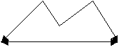
The figure on the left is monotone with respect to the y-axis while the one on the right is monotone with respect to the x-axis.

Some non-convex polygons can also be monotone (with respect to some line)

It has been proposed that an algorithm finding the C-Space of a monotone robot would have O(mn²).

M: Monotone Polygon with m edges

N: Multiply Connected Workspace

MH, NH: Convex hulls of M, N

I(P,Q): Set of all configurations of P for which P does not intersect ext(Q)

E(P,Q): Set of all configurations of P for which P intersects int(Q)

The polygons in NH/N are the concavities and holes of N. Let T be the set of triangles obtained by triangulating NH/N.

Then I(M,NH) = I(M,NH)/U_D'T E(M,D)

Because MH is convex, I(MH,NH) = I(M,NH)/U_D'T E(M,D)

ALGORITHM

Input: A monotone polygon M and a polygon N

Output: The boundary bd(I(M,N)) of the set of all placements by translation of M inside N.

Step 1: Compute the convex hulls MH, NH O(m),O(n)

Step 2: Determine I(MH,NH) O(m+n)

Step 3: Compute T O(n lg n)

Step 4: Determine E(M,D) O(mn log n)

Step 5: Compute I(M,N) = I(M,NH)/U_D'T E(M,D) O(mn²)