LOCAL RULE

GLOBAL METHODS: Try to capture the global connectivity of the robot's free space into a condensed graph that is subsequently searched for a path. They are based on searching procedures and could churn out paths that optimize the path length. The planning methodology involved further representation of the environment models in terms of suitable data structures such as graphs, trees so that finding a path in the workspace is equivalent to searching for a route between two nodes on the graph

LOCAL METHODS: The values and actions are not dependent on the distribution and shapes of the C-obstacles beyond some limited neighborhood of the current configuration/position of the robot. Real-time navigation strategies came up as a consequence of having to cope with pragmatic realities such as inaccuracy of environment models and the requirement of the robot to navigate in unknown and unstructured environments. These approaches generate a linear and angular speed during every sample instant as a combination of the response outputs for different behaviors such as obstacle avoidance and target reaching. The path generation is obtained by advancing the robot to a new position and by repeating the process.

A genetic algorithm is used for developing an optimal fuzzy logic controller. This effectively converts an online path planning problem to an offline optimization problem. The scheme is depicted in fig. 1.

Instantiations of the control strategy to be implemented online are randomly generated and act as individuals for the GA population. The GA then optimizes the control strategy offline. The optimized rulebase as obtained by the GA is then used online for path navigation and obstacle avoidance. This allows the computationally intensive optimization to be done offline and leads to an efficient online implementation that gives an optimal path, yet which is able to do it in real-time and only using the scarce memory and computational resources available on an autonomous robot.

The rules were represented as a set of condition-action pairs. The first condition is the distance of the nearest obstacle forward from the robot. Here forward means within the field of view of the robot. As our obstacles are square shaped, the distance is calculated from the line joining the current position of the robot to the point of intersection of line joining the robot to the center of the obstacle and the nearest edge of the obstacle. The second condition is the angle between the path joining the robot and the target point and the path from the robot to the nearest obstacle forward. The action is represented by the angle of deviation for the robot from the path joining the robot to the target point. This is depicted in fig. 2.

Fig. 2. The input (distance and angle) and output (deviation) variables of the fuzzy logic controller

Thus angle and distance form the fuzzy inputs and deviation forms the output. Here the fuzzy values for distance, angle and deviation are depicted in fig. 3.

Fig. 3. The fuzzy membership functions for angle and deviation (left) and distance (right)

Triangular membership functions were used with the relative spacing of the membership distributions being constant. The membership functions were kept same for angle and deviation. The fitness of the individual is determined as a function of the total time taken by the individual to reach a predetermined goal in each of the one hundred cases considered. Suitable penalties are imposed, if the robot collides with an obstacle, is not able to reach the goal in the allowed maximum time or goes outside its work area. In each of the cases, the desired number of obstacles is positioned randomly on the workspace. During the optimization of the fuzzy logic controller, our aim is to minimize the total time taken. For this the time is suitably converted to fitness values. A count is also made for each individual (rulebase) of the number of cases for which the robot is successfully able to reach its goal. Thus a perfect individual would be the rulebase using which the robot is successfully able to reach its goal in all the cases in a near time optimal manner. In this context our proposed hybrid algorithm is successfully able to solve each of the cases in a time optimal manner.

RULEBASE REDUCTION

The evolved models of the optimal fuzzy logic controller (even the perfect individual) were complicated and included a large number of rules that seemed redundant. The evolved optimal rulebase for cases when the number of obstacles was changed to 8, 16, 32, 40, 64, 128 and 256 came out to be different. This should not be the case as ultimately the final rulebase to be implemented on the robot would be unique irrespective of the number of obstacles in the environment. After all if one can know the number of obstacles in an environment, one can also know their position and then the environment is no longer unknown!!

Local search is performed on the optimal evolved rulebase that is able to solve all the cases. Each of the possible subsets of the evolved rulebase is tested and its fitness evaluated. Typically the rulebase consisted of seven to nine rules.

The rulebase was evolved with a test-bed of 100 different cases. Each case has 40 obstacles of which 10 were placed on the path joining the start point of the robot to the end point. Here the workspace was of size 80x80 with the initial point being the origin and the goal point being (76,76). Goal was attained if the robot came within unit distance from the goal.

The GA evolved the perfect individual after 1581 fitness evaluations. The population size of GA was kept 100, mutation probability 0.02 and crossover probability 0.9. Length of the string was kept 45 with the maximum number of allowed rules in the rulebase being fifteen. The evolved rulebase is shown in table.1. Here the first rule can be interpreted as: if the distance of the nearest obstacle forward from the robot is very near and the angle between the line joining the current robot position to the goal point and the line joining the current robot position to the center of the obstacle is left, then the robot should not deviate and go ahead.

Distance	Angle	Deviation
Very near	Left	Ahead
Very near	Ahead left	Ahead right
Very near	Ahead	Right
Very near	Right	Ahead left
Near	Left	Right
Near	Ahead left	Right
Near	Ahead	Right
Near	Right	Ahead right
Far	Ahead	Right

However when we apply local search, the rule base is shortened to the one given in table.2. This was due to the redundant rules that were present in the rulebase evolved by the GA got eliminated by using local search. The number of rules in the rulebase is reduced from nine to four without any reduction in the fitness. Both of the rulebase are able to solve all the 100 cases in 11738 seconds, thus taking on an average 117.38 seconds for each case as against the allowed maximum time of 400 seconds.

Distance	Angle	Deviation
Very near	Right	Ahead left
Near	Ahead left	Right
Near	Right	Ahead right
Far	Ahead	Right

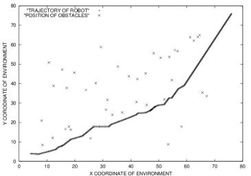
Fig. 4. The position of obstacles and the path of the robot obtained using the shortened rulebase

Thus we see that the robot is able to effectively navigate through obstacles and reach its goal. The path of the robot in the other ninety-nine cases is similar to the above curve and proves the efficacy of the technique.

FUZZY APPROACH COMBINED WITH PERCEPTION AND REMEMBRANCE OF THE ENVIRONMENT [2]

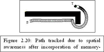
lack of memory-based behavior and reasoning is apparent in most of the algorithms and their absence become prominent during certain aspects of navigation like the robot's failure to get aware of local minimum traps.

The input to the target orienting module is the difference angle mentioned in section 2.2. The output of the module is denoted as, or the turn angle of the robot (angle by which it must turn) due to the target reaching behavior. It is that behavior responsible for orienting the robot towards its target.

Rules : (i) If target is on the left then turn left (ii) If target is on the right then turn righ

1. If the object is detected at near ranges on the left then turn the robot right by a large angle.

2. If the object is detected at far ranges on the left then turn the robot right by a small angle.

Hence the net change in orientation of the robot is considered as an weighted sum of the changes in orientation due to the individual modules. The weights ascribe the proportion of importance to the individual behaviors.

Other specialized modules like wall following and sampling behavior also present

Fig 8. Flow diagram representation of real-time navigation with the primary modules alone

Adaptive fuzzy control where the parameters of the rulebase get tuned through a learning mechanism to obtain the desired performance or the desired input-output mapping through a network structure decides the parameters.

RIGHT SENSOR	CENTER SENSOR	LEFT SENSOR	CLASS
VERY NEAR	VERY NEAR	VERY NEAR	0
NEAR	NEAR	NEAR	1
NEAR	NEAR	FAR	2
NEAR	FAR	NEAR	3
NEAR	FAR	FAR	4
FAR	NEAR	NEAR	5
FAR	NEAR	FAR	6
FAR	FAR	NEAR	7
FAR	FAR	FAR	8

A double layered network for spatio-temporal classification, which enables the robot to understand as well as remember the various scenarios encountered during its navigation is used. At the first layer fuzzy rule-base does the spatial classification and at the second layer SOM and Fuzzy ART network is used for temporal learning. The SOM captures to a reasonable accuracy the size and shape information of the obstacles or landmarks in the environment and provides stability to the network by accurate recall of previously stored patterns but is not plastic enough to new situations. The online classification property of Fuzzy ART however makes the network plastic to new patterns but its ability to interpret the environment is poor when compared to the SOM. Hence we use both the SOM and the ART in the second layer to avail the advantages of both.

A navigating robot understands its environment in terms of landmarks. A landmark such as a corridor can be considered as an experience of a temporal sequence of sensory patterns and represented in terms of such spatio-temporal patterns. Since remembering a moderately long traversal involves storing several instants of sensory data resulting in huge memory requirements, a classification scheme is essential for classifying the spatio-temporal data into meaningful information. The spatio-temporal classifier network does this.

In the proposed scheme spatial understanding is achieved through the weight vectors of the neurons that are codified representations of the local space of the robot. Storing the lattice positions of the winning neurons during a traversal enable storage of the comprehended scenarios while choosing a particular lattice position achieves focussing on a particular remembered experience. And temporal correlation of a particular experience occurs through recall when the neuron coding that experience gets activated more than once during traversal.

A landmark is modeled as an experience of spatio-temporal patterns. Each sample of such a pattern consists of range readings obtained by the seven sensors. For reducing complexity of storage, representation and learning a long sequence of such samples, each sample is mapped to a class by the fuzzy classifier. The number of such classes in a temporal sequence is fixed at 3 with no two consecutive classes being identical. The minimum number of times each class must occur in a sequence to filter noisy samples is termed the lower bound for that class. The structure of the double layered classifier network is shown in figure 9.

The structure represents the process of extracting the temporal order of the classes before giving it to the second layer. As discussed in the previous paragraph any two consecutive classes in the final sequence to be classified must be different. The comparator (figure 2.16) which compares the present class C(t) with the class of the previous instant C(t-1) does this. When the compared values are different C(t-1) is extracted to form the first class in the sequence to be classified by the second layer. The process is repeated and when three such classes are extracted the sequence, y1, y2, y3 (see figure 2.16) is input to the second layer of the classifier.

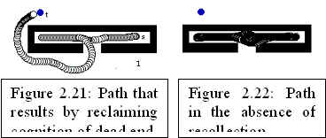
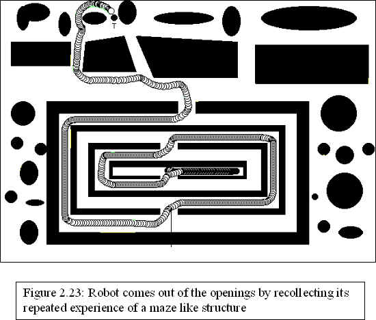
Consolidated understanding of the environment is that spatial understanding derived by considering a sequence of preliminary spatial understandings ordered in time. . The sequences are obtained by navigating the robot across landmarks typically encountered in indoor environments. These sequences are reduced to a sequence of 3 classes and presented as inputs to be learned by the temporal classifier (fig 9). The SOM is trained over these sequences of classes. On encountering a sequence of patterns that represents a particular landmark the neuron in the lattice is triggered and the robot becomes aware or cognizant of the presence of such a landmark in its vicinity.

Fuzzy ART is capable of learning new patterns and simultaneously remembers the earlier patterns to a reasonable accuracy. It eliminates the need for maintaining a map of large neurons most of which are idle. The ART network can dynamically add new patterns according to the local environment of the robot and can afford to forget patterns that have not come within a recent time interval, say in the last hundred samples of the environment thus memorizing the environment to the extent needed.

. As the robot navigates through the environment the sensory inputs are obtained and classified by the first layer of the classifier network. The temporal order of classes is extracted. A sequence of 3 such classes with no two consecutive classes being identical forms the input vector for the Fuzzy ART. The Fuzzy ART maps the sequence with an earlier one or adds a new spatio-temporal pattern to the existing set of patterns. The decision for adding a new pattern is decided by the vigilance parameter, which is set to 0.9 in our algorithm. A review of the Fuzzy ART algorithm had been given in the previous section.

1. Pratihar, D.K.: Path and Gait Generation of Legged Robots Using GA-Fuzzy Approach. PhD Disseration, Department of Mechanical Engineering, Indian Institute of Technology – Kanpur, May 1999 (1999).

2. Krishna, K. Madhava: Soft Computing Applications to Real-time Navigation of a Mobile Robot in Stationary and Dynamic Environments. PhD Disseration, Department of Mechanical Engineering, Indian Institute of Technology – Kanpur.