presentation by Anusheel nahar

OVERVIEW OF PRESENTATION

. controlability with non holonomic inequality constraints
. implementation using grid decomposition for car like
  and tractor trailer robot satisfying  non holonomic inequality constraints
. implementation for a NHR on a natural 3-D surface like a planetary rover
. jumps for a point NHR using CSC curves
. planning method using jumps
. shortest path accessibility region for a car like robot that can only move forward
 

what does a non holonomic constraint mean?

. tangent space(ie set of velocities) of parameters constrain the motion of robot such that
  the resulting dynamic equation is non integrable with respect to time .
  e.g a car like robot cannot move perpendicular to its main axis
  tangent space dx/dt .sin(theta)=dy/dt .cos(theta)
  x= xcoordinate of centre of rear axle midpoint
  y= ycoordinate of centre of rear axle midpoint
  theta = heading angle of the car

how does NH equality constraint  effect the state of the robot ?
.NH equality constraints reduces the dimensionality of the configuration space
.if there are k constraints then the dimensionality is reduced by 1 per constraint
 

non holonomic inequality constraints
. A car like robot has 2 parameters that govern its motion/position
  velocity of rear wheel v
  steering angle  phi
. for most real cars the steering angle is constrained
 -phi max< phi < phi max

+ve = left turn
-ve = right turn

. radius of turn
  R= front_rear wheel axle seperation/tan(steering angle)=L/tan(phi)
  Rmin=L/tan(phi_max)
 (velocity of car along axis)/R= d(theta)/dt
 (dx/dt)^2+(dy/dt)^2=(R*(d(theta)/dt))2>=Rmin^2*((d(theta)/dt))2)
so the constraint
 (dx/dt)^2+(dy/dt)^2-Rmin^2*((d(theta)/dt))2)>=0

how does a non holonomic inequality constraint effect
.it picks up a subset of velocity vectors (x' , y', theta') from the m-k ie (3-1 )
dim  tangent  space for the car like / (4-1)tractor trailer robot which satisy the constraint
 

controllability with inequality constraints
.for a  car like robot the 2 constraints mean
 1. it cannot move sideways
 2. it cannot move on a radius less than R_min
.if we can define manuevers which lead to destinations without violating 1
 and 2 then we are done.
 then given a obstacle free world we can reach any configuration to any other
 just like a free moving robot having 3 degrees of freedom
formal proof  :refer book

manuever 1

 

1.consists of 3 segments
   -arc of radius = R_min (left) angle =delta theta
   -straight line tangent to the circle1 symmetric about the initial pos(in rev gear)
   -arc of radius = R_min (right)        =delta theta
   sideways distance moved= 2*R_min*(1/cos(delta_theta)  -1)
   this manuever can be made sufficiently small in terms of the distance moved sideways
   by reducing delta_theta.
    this mitigates the effect of constraint 1
 

2. any amount sideways movement can be acheived by concatenating sufficient
   no. such manuvers(however small).

manuever of type 2

.consists of 3 segments
    - arc of radius(R_min)  by delta theta say towards right
    - segment in rev gear
    - arc of radius(R_min)  by delta theta towards right
angle rotated= 2*delta theta

any amount of rotation can be obtained by the above manuver so effectively
mitigating constraint 2

IMPLEMENTATION FOR A CAR  LIKE ROBOT

approach1
generate a path ignoring the NHC using normal methods like PRM ,potential fields and then try to convert it using the above manuvers .
-by simeon and laumond

problems
-very expensive
-unreasonable paths obtained

approach2
generate a set of corridors along which the robot can safely travel and
use the above curves for transferring between the corridors

problems
-generally very difficult to define a set of corridors in a workspace
- inefficiencies while trying to add various interacting curves to get a global solution

approach3
task: reach (x2,y2,theta2) from (x1,y1,theta1)

governing equations
1.x' = v * cos(theta)
2.y' = v * sin(theta)
3.theta' = v/L * tan(phi)
v = speed along the axis
theta = heading angle

on integrating we get
theta(t)= theta(0)+ v/L*tan(phi*t)
x(t)=x(0) + L/tan(phi) *(sin(theta(0)+v/L *tan(phi))-sin(theta(0))
y(t)=y(0) - L/tan(phi) *(cos(theta(0)+v/L *tan(phi))-cos(theta(0))

1. discretize and divide the space (x,y,theta) into  3D m*m*m cells grid.
2. we take t=1 and try to integrate along small paths in the grid
3. we use the parameters v,phi for searching
  given a node we generate next 6 nodes s.t
    (v,-v)*(-phi_max,0,phi_max)
   ie forward Fw, forward left FwL ,forward right Fwr
   and similiarly for backwards  Bw,Bwl,Bwr
   and integrate the selected pair on a small path t=1 by putting in the integrated eqn

assumptions
1. robo has only 2 velocities +-v
2. we consider it to go only least radius

4. maintain a tree
   a.  start node = x1,y1,theta1
   b.  add the 6 following nodes in the tree and mark them on the grid as visited
   c.  generate subsequent 6 and so on
   d. if a node corresponds to intersection discard the branch
   e.  if a node is already visited discard it
   f.  do so till the cell where the goal is  reached
   g  the nodes can be added in sorted order in terms of a cost function
 

5. issues
.  time is taken as 1
.  velocity =2*length of a grid element so as to prevent the robo to stay in the
   same cell on any motion and also to prevent it from going into a cell
   farther than 2 cells (this could lead to collision detection misses)
.  cost function = no.reversals  (gives too long path)
.  good cost function based on both time and reversals

6.results
.   good results for parallel parking problem and small maps
   with 128^3 cells
.  also good for solving locked steering problem
 

7.complexity
   expensive   O(m^n * log(m^n))
   m = cells per dimension
   n  = dimensionality of the space

EXTENSION TO TRACTOR TRAILER PROBLEM
1.
   governing equations of the model
   x1' = vcos(theta1)
   y1'=  vsin(theta1)
   theta1' = vtan(phi)/L1
   theta2' = v/L2 *sin(theta1-theta2)

   L2= wheel seperation of trailer and rear wheels
   theta2= heading angle of trailer
 

2. last equation is non integrable . solved by numerical methods

3.results for 64^4 discretization

IMPLEMENTATION FOR A PLANETARY ROVER ON A 3D SURFACE

1.introduction
   -6 wheeled robot on a 3D surface
   -having 6 degrees of Freedom
    (x,y,z),(roll,pitch,yaw) of the main frame of the robo
    you control the torque on each of the wheels

2.dimensionality
6+n(due to kinematic/dynamic/friction  constraints of surface/wheel interactions) dim space causing heavy computation time
 

3. constraints
    -geometric obstacles which u have to avoid at all costs
    -other bad areas which may be entered into but will effect the performance of the
    robo like slippery areas
    - some wheels have always to be on the ground
    - non holonomic constraints

4.use 2stage approach to find a safe and executable path
 -  first generate a global path satisfying geometric constraints
 - locally optimize on it
 

5. modelling of the robot
- grid of interacting rigid objects satisfying newton / euler equations of dynamics
- these objects connected by connectors modeled on dampers  and springs.
- e.g model a revolute joint as 2  pairs of points 1 in each part along the axis of the joint

6 modelling of surface
- as a grid of points with each point being at a centre of a non elstic sphere
-the surafce as envelope of the spheres
- these points are governed by viscoelastic laws modelled using dampers/springs/masses
   etc
 

7 geometric path palnning
  reduce the problem to 2-D  carlike
  .ignore terrain effects now
  .similiar to the above graph search method
  .except instead of taking v,phi,t constants we do the following
  v= ev*v_max
  |phi|=ep*|phi_max|
  ev<1,ep<1
   and keep them constant for a short path. so you on a radius > min radius
   t  is chosen such that atleast 1 grid cell is moved in 1 step of node generation.
    cell size= 1 robo length in this case.

8.cost function
   takes into account the past and the futurejean daniel boissonat
   euclidean distance may be used
   but distance of a curve like C1SC2 circle-segment-circle can be used

9.dynamic motion planning
  aim
  .smoothness
  .ensure that the robot can execute a safe path
 .the robot may need to stop at certain points and manuver
     to ensure passage on certain types of terrain. all this makes exact path prediction very difficult

to overcome these we see that
there are 2 kinds of points
  1. manuevering points where  the steering angle changes . velocity < v_max( radius of     curvature,terrain)
  2. straight paths where angular velocity is nearly 0

10 actual physical  planning
1. generate a path of CSC type on a local scale
2. try to apply certain control torques on the wheels at each incremental steps and analyse
    the surface wheel interactions based on the model. this will show up the                       sliding    interactions  as well and the robo may drift away from the nominal path
3. assume v and theta to be constant during each time step delta t
4. if the robot goes too far from the desired path of CSC type we discard that node and apply
   another control torque to the wheel and do it till a nearly good path is obtained
 
 

JUMPS

modeling

. the NHR can be modelled as a point robot with x,y, theta by appropriately
    growing the obstacles
.given a obstacle free world
   a NH robo can reach any configuration to any other by executing
   a curve of CSC type with radii of circles  being  the min turning radii
. 4 types of curves
  1. Left -Left LL
  2. LR
  3. RR
  4. RL            where the sequence shows the directions of the 2 circles of min turning radius

 a semi free path  (one that touches the obstacles atmost at a finite no. obstacles)
can be broken into a no. subpaths.
-each can be further broken down to represent a jump recursively if the whole does not
  lie in the free space.
-we eliminate subarcs lying entirely in free space by translation
   longer than R_min*pi are made equal to R_min*pi  which may in turn touch an obstacle
   shorter ones may be reduced or made into straight lines. thus a semi free path consisting
   of only jumps can be obtained . which is executable.
 

algo
jacob and canny
1.we make a set of nodes s.t
    if it is a vertex of a polygon then we consider (x,y,theta(k))
    where k= 0,1,2.... 2*pi/delta-1
2. divide each edge into some no. points
    the robot can slide along it only in 2 directions +-theta(e)
    include the node (xl,yl,+-theta(e))
3. 2 nodes are connected if  using a directed jump we can reach from a start to a goal
4. path planning can be done by searching the graph and using some cost function

assume n(e)=linear fn of (1/delta)
no nodes = O(n/delta)
graph building =O((n/delta)^2)
collision check for each jump=O(n)
time complexity= O(n^3/delta^2)
 

**efficiency can be improved by not counting nodes which represent vertex and point inside
 the obstacle /or is diagonally opposite to such

better use of jumps by using jump graphs

O((nlogn+1/delta)*n^2/delta)

comments on motion of a car like robot modeled as a point that can only move forward
1.put origin on robot
2. let robo point in positive x axis
3. make circles corresponding to left and r

LS=left straight
LR=right left on (circles)

we consider only +ve y plane .for -ve plane the story is symmetric
to move to a point in  x>0 and lying outside the circle
.LS is optimal path

.for path on circle L is best

.for path inside the circle x>0
 RL is best

.for path on/inside circle on x<0
 RL is best

.for others LS is better
 

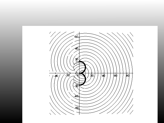
d= distance of the optimal path
which can be used to draw the iso distance lines

the arcs x>0 act like a wall the lengths for pointsjust inside and just outside are vastly different
LvSo
distance=pV
v= angle travelled in left arc

RLv
=p(2pi-v+2/3(pi-v))

applications for
modelling car chasing problems

 
 
 
 
 
 
 

references
1.jean daniel boissonat INRIA       here
2.cherif laugier              INRIA