I
I
Fig 1. Input to the algorithm Fig 2. Output- the visibility graph
Input: n line segments
Output: visibility Graph
Notation used:
S:- Set of n line segments
Gs = (Vs, Es) - Visibility Graph
s(v) - segment to which v belongs
d(v,v') - direction from v to v'
Ds - sorted set of directions d(v,v')
s(inf) - line segment at infinity
v(inf) - vertex point at infinity
S(inf) - union of set S and s(inf)
R , a subset of Vs x S(inf) -
It is a view relation that stores the pair of segments and the vertices
(v,s(v)) s.t. s(v) is the segment visible from vertex v along a direction
d
The algorithm improves the complexity by reducing the time taken to sort directions d(v,v') to generate Ds
Idea behind the Algorithm:
The algorithm is a variation of the sweep-line algorithm and like it, works by rotating a line updating information about the topology of vertices, building the visibility graph in process. The information is stored in a relation R. The bottleneck in this approach is the sorting of the directions in which the line needs to be rotated.
Fig 2. This figure shows the initial relation R0
for a set of segments.
The dotted line from each vertex v points to the segment
s,
for which (v,s) belongs to R0
The algorithm circumvents this problem by avoiding to sort the directions. Rather it uses a permutation of them which can be computed in lesser time and serves the same purpose.
When we rotate the sweep line, the relation R0 does not change till we reach the next direction in Ds. Even then, the relation changes locally. There are four cases possible.
Fig 3: These are the four cases that can arise in sweep line
rotation.
In case (i), No edge needs to be added to the graph.
In case (ii), the edge from v to line 2 is added to the graph.
In case (iii), the edge from v to line 2 is added.
In case (iv), no edge is added.
INITIALIZE R0:
for every point v belonging to Vs, let (v,s) belong to
R,
s.t. s is the first line intersected by the ray emanating from v in the
vertical direction downwards.
UPDATE R:
if s(v') = s(v) then /* case (i) */
edge(R,d) = phi and rot(R,d) = R;
else if length(vv') < length(vw) /* case (ii)
*/
edge(R,d) = {{v,v'}} and
rot(R,d) = R - {(v,R(v))} +
{(v,s(v'))};
else if s(v') = R(v) /* case (iii) */
edge(R,d) = {{v,v'}} and
rot(R,d) = R - {(v,R(v))} +
{(v,R(v'))};
else if length(vv') > length(vw) /* case
(iv) */
edge(R,d) = phi and
rot(R,d) = R;
ALGORITHM:
INITIALIZE R0
Es = phi ; R = R0
for i =1 to (2n C 2) do
UPDATE R;
Es = Es U
edge (R,di)
R = rot(R,
di);
end;
Independent Directions : Two directions d =
d(v,w) and d' = d(v',w') are independent if {v,w} intersection {v',w'}
= phi.
Independent directions have a special property that if we change two consecutive independent directions in Ds, Es is still computed correctly.
Thus, instead of using the sorted set Ds, we can use a permutation of Ds, obtained by interchanging independent directions, called a "good permutation".
Good permutation can be computed in O(n^2) time!!!
Computation of good permutation of Ds.
Complexity of algorithm is O(n^2).
GENERALIZED POLYGONS
A generalized polygon has following properties
Types of generalized polygons
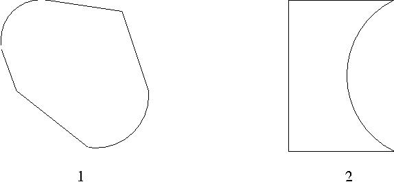
Fig 4. Convex generalized polygon
Fig 5. Non-convex generalized polygon
Reduced Generalized Visibility Graph:
The reduced generalized visibility graph consists of
VISIBILITY GRAPHS IN THREE DIMENSIONS:
Papadimitrou gave an approximation algorithm
of polynomial time
Given a positive real number e, it returns path whose length is at most (1+e) times the shortest path length. The algorithm works by dividing the lines into segments and constructing an approximate visibility graph using these segments as nodes.
The NP-hardness of the problem arises out of the difficulty faced in finding out the distance between two line segments in three dimensions.
ALGORITHM:
1. Divide all edges of the C-space of obstacles
into several segments.
2. The segments are assumed to be small enough to approximate
the distance between the a pair of segments as the distance between the
mid points of the segment.
3. Using segments as nodes, a visibility graph is constructed
where two nodes representing a pair of segments are connected if they are
visible to each other.
4. After the construction of the graph, standard graph
search algorithms are used to search for a path.
Computation of Visibility Graph:
For a pair of lines dividing into segments, fix a coordinate system (x,y) s.t (a,b) represents the path segment on line 1 and both segment on line 2.
This reduces the problem to that of finding a region R, which represents pair of segments visible to each other.
R is calculated using advanced coordinate geometry , which is a union of hyperbolic regions.
Once, R is calculated, the visibility graph is constructed by traversing the boundary of R, and for all points (a,b) belonging to R, joining the nodes representing a-th node and b-th node by an edge as they are visible to each other. Invisible segments are not joined in this manner.
Path is obtained by searching through this graph.
Complexity of the algorithm is O(n^4(L +log(n/e))^2/(e^2))
CONCLUSION:
REFERENCES: