Methodology
Besides input and output format and implementations, which
are discussed at length in Implemenatation Details link, our project mainly
consists of implementation of Genetic Algorithm to optimize the placement
problem. In order to avoid ambiguity, and convey a clear picture of our
procedure we have divided our methodology in the undergiven divisions-
-
Basic GA outline
-
Population Generation Scheme
-
Basic GA operators and their implementations
-
Penalty functions
-
Objective function
-
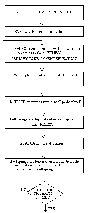
Flowchart Representation of the problem
BASIC GA OUTLINE:
GENETIC ALGORITHM
is
a random search method best suited for optimization and search problems
involving large database. This evolutionary algorithm is based on Darwin's
"Theory of Evolution". In this evolutionary algorithm, initially we
code the variables of the function to be optimized in form of a chromosome
. Then, we generate initial population randomly for the solutions of the
function. Using GA operators like selection, crossover, mutation etc. (
discussed below ) we keep on maintaining diversity in the generated population
and keep heading towards goal by keeping in the population only the fittest
individuals. Generation number, population size, crossover probobality,
mutation probability and convergence limits are some of the parameters
of GA which are to be carefully chosen for the GA to converge.
Since, our cell placement problem involved handling
of large data and time was also a crucial factor we chose this evolutionary
algorithm for our NP Complete problem.
POPULATION GENERATION SCHEME:
Our souce code has in-built Random number generator
to generate the initial population randomly. The generator is borrowed
from Goldberg, and uses Box-Muller method to maintain the deviation
between the random numbers generated. It takes initial random seed number
and then generates the entire population by initiating the randomization.
Random function chooses randomly a number between 0 and 1 using Subtractive
method and then generates the specified number of population individuals.
BASIC GA OPERATORS AND THEIR
IMPLEMENTATIONS;
For the algorithm to maintain diversity
in its population data base and to head towards the optimal solution continuously
it relies on several operators, named on Evolution line,as discussed below-
-
ENCODING
In order for the algorithm to proceed
we need to encode each individual of the population so that GA operators
can operate on it to genarate solutions. Though Real Genetic Algorithm
can also be used but we are using Binary GA in which we are encoding
each individual as a chromosome of bit pattern consisting of 0's and 1's.
An exmple illustrates this,
e.g.
Suppose x=100, y=65, oriientation=1(correct).
We will represent this solution using eight bits for x and y and one for
orientation as,
01100100-01000001-1
Suppose 3 cells are there and there
( x , y , orientation ) are as ( 30 , 23 , 1 ), ( 30, 13 , 0 ), (
30, 3, 0 ) respectively and each are of dimension 10x10 then the
binary chromosome used will be,
11110-10111-1-11110-01101-0-11110-00011-0
-
SELECTION
In order to select two individuals
from the population for reproduction, to produce offsprings for the new
population an elaborate scheme has to developed so as to produce healthy
offsprings. The selection operator may be implemented in algorithmic form
in number of ways like Roulete Wheel Selection, Stochastic Universal
Selection, and Binary Tournament selection. Roulette selection
is the easiest method but for our placement problem it has been found that
Binary Tournament selection gives the best results, so we have implemented
this selection scheme. In BTS, two individuals are taken at random and
the better individual is selected from the two. In our scheme we are not
allowing the replacement so the two individuals previously selected are
set aside in the next selection operation. Since two individuals are replaced
from the population for every individual selected, and population size
remains constant from one generation to the next, the original population
is restored after the new population is half filled. Therefore, the best
individual will be selected twice, and the worst individual will not be
selected at all. The number of copies selected of any other individual
cannot be predicted except that it is either zero, one or two.
-
CROSSOVER
Once two chromosomes are selected,
the cross-over operator is used to generate two offsprings. It can again
be of several types like one-point crossover, multi-point crossover,
and uniform crossover. We are implementing one-point crossover which
is simplest and for our problem as good as any other schema. In this scheme,
a point is selected at random in two selected chromosomes and their contents
of left and right of that point are crossed or interchanged. Crossover
takes place generally with some probability which is kept high.This is
illustrated by the example here,
e.g.
Parent1: 101101101
/ 111001100
Parent2: 001101100
/ 100101000
Offspring1: 101101101/
100101000
Offspring2:
001101100/ 111001100
Explaining this operator in context
of the placement example mentioned at start is,
Parent1: 1011010101010001110010/11110000110
Parent2: 1111010111111110011010/11001011010
after crossover,
Offspring1: 1011010101010001110010/11001011010
Offspring2: 1111010111111110011010/11110000110
Offspring1 as found above is one
of the optimum placements.
-
MUTATION
As new individuals are generated,
each character is mutated( changed ) with a given probobality which is
generally very small in order to maintain the identity of the individuals
to a great extent. This operator is employed to maintain diversity in
the generated population so that search can span over large and otherwise
unexplorable area. The action of this operator is shown below through an
example,
e.g.
Before: 11010011001
After :
11010111001
In this it is seen that mutation
has taken place on the sixth bit.
Continuing again our initial example, suppose one of the
individuals is,
Before:111101011111111001101011110000100
After mutation at 32nd bit we get,
After: 111101011111111001101011110000110
-
FITNESS EVALUATION
In evaluation, each individual
is tested for the solution and given reward if is good and penalty
otherwise. After this the individuals are ranked on the basis of their
points and of them top ones according to population size are taken while
the rest are dicarded. This is called an Elitist model of GA.
e.g.
For the example of placement considered,
Offspring2 generated above when evaluated satisfies all the criterion of
no overlap , interconnect specifications satisfied, and area is small
so GA returns high fitness value for this individual.
-
STOPPING CRITERION
There is some point at which GA
must stop its execution whether it finds the solution or not. This is ensured
by the stopping criterion. The GA stops its execution if it finds the required
value specified for the objective function, or number of generations as
specified are over or the population individuals are too much spread so
that GA is unlikely to converge. These criteria which help GA to stop are
collectively called Stopping Criteria.
PENALTY
FUNCTIONS:
In order to avoid the overlap of the cells to be
placed and the cells with large number of interconnects to be placed far
apart we have given penalty for these two cases. These two penalty functions
have been discussed below,
-
OVERLAP PENALTY
This penalty is given to avoid the overlaps and is directly
proportional to the amount of overlap.We calculate the overlap area and
then multiply it by a scalar factor to give corresponding penalty. For
this we see if difference between the x-cordinates of two rectangles concerned
is less than half of the sum of dimensions of those rectangles along x-axis
then these rectangles are overlapping along x-axis. Now if two rectangles
are overlapping in x-axis as well as y-axis then such placement is unwanted
and we give a penalty for it . For calculating penalty we find the x-overlap
and y-overlap and multiply it to get net overlap area and accordingly give
penalty. If the cells are completely overlapping then we give slightly
higher penalty by exaggerating the overlap area.Penalty function for overlap
can be written as,
Over_penalty = ( x-overlap * y-overlap ) * weight_factor
where x-overlap and y-overlap are defined
as the difference between centres less half the sum of the dimensions in
that direction.

e.g.
Suppose we consider one unoptimized individual with overlap
for the example being continued as,
Individual: 11110-10110-1-11110-01100-0-11110-00011-0
if weight factor is set as 50,
between cells 2 and 3 there is overlap,
x-overlap=10
y-overlap=1
thus Over_penalty returned= (10*1)*50=500
-
INTERCONNECT PENALTY
We know the number of interconnects between each cells
which is the netlist, so it is intutive to place two cells with large number
of interconnects adjacent to each other. Now if our GA generates a solution
where such cells are placed wide apart then we give a penalty for it
so as to discourage such placements. Penalty is given on the basis of number
of interconnects between the cells and overlap along any axis.If the cells
overlap then no interconnect penalty is given.Suppose the individual turns
out such that cell1 and cell2 are adjacent to each other then the magnitude
of the penalty for interconnect can be written as,
Inter_penalty = ( netlist * x_over ) + ( netlist *
y_over ) (summed over all pairs of cells)
e.g.
For the individual string considered above for
overlap penalty suppose,
interconnects between cell1 & cell2=10
interconnects between cell1 & cell3=13
interconnects between cell2 & cell3=0
then inter_penalty=((10*(-10))+(10*(-10)))+0+0=-200,
the negative penalty factor implies that the placement
is good as far as the interconnects are concerned.
OBJECTIVE FUNCTION :
After generating the centres of the cells through
GA, we see the orientations of each cell and determine the co-ordinates
of the vertices of the cell. Then we see maximum and minimum co-ordinate
along each axes and find the Chiparea as,
CHIPAREA=
(MAX(x) - MIN(x) ) * ( MAX(y) - MIN(y) )
Since our GA minimizes the objective function,
so chiparea must form part of it, also we don't want cell overlaps
and interconnect mismatch so we add the penalty to chip area with
weights so that objective function is increased if there are any unwanted
conditions. So our net objective function which GA minimizes is,
OBJECTIVE=
CHIPAREA + ( Over_penalty * weight1) + (Net_penalty * weight2)
By giving appropriate weights we ensure that area
minimization is our prime concern but there mus be no overlap at all and
minimum amount of interconnect mismatch. So, we give maximum weight to
overlap and least to interconnect mismatch.
e.g.
For the string considered in the Penalty section,
Chiparea=290
Over_penalty=500
Net_penalty= -200
Now if weights for over_penalty and Net_penalty
are 2 and 1 respectively then,
Objective= 290 + ( 500 * 2) + ( -200 *1) = 1090
FLOWCHART OF GA:

*********************************
MAIN

