ME751 Project Report: Learning Tolerance Models
Computer Aided Engineering Design ME 751/451 Jul-Nov 99
-:Mukerjee
Learning Tolerance CAD Models using PCA
|
Gagan Deep Arora (96095)
Ravi Prakash Srivastava
(96226)
Indian Institute of Technology - Kanpur : November 1999
Contents
In Addition...
- Original Proposal for this work
- Preliminary Presentation (power point format)
- Various Codes used in the Study
Motivation
Actual Design Process involves assignment of shapes and their dimensions which
in turn serve as the guidelines for the manufactureres, developers, users, and
the designers themselves. The various stages of development of a design,
particularly the machinig fabrication and testing involve considering it as
an approximation in the sense of defining tolerances for both shape and size
parameters. These tolerances are inevitably encountrered due to the limitations
of each of the stages of the design and development process. It is therefore
only essential that the designer be equipped with tools which allow him to
design and test with real-life considerations of tolerances.
The present-day CAD tools have little to offer in this area and much work needs
to be done before tolerances can be handled by CAD platforms which can
identify shape classes rather than rigidly considering shapes alone.
The present work is a step in this direction wherein we attempt to extract
toleranced CAD models from images of simple, yet representative, 3-D models
and providing a shape class for the identified shape.
![[Back to Top]](images/icons/first.gif)
![[Previous]](images/icons/prev.gif)
![[Next]](images/icons/next.gif)
![[Last]](images/icons/last.gif)
![[Home]](images/icons/home.gif)
![[Information]](images/icons/info.gif)
Problem Statement
The problem taken for the current study hovers around the central idea of introducing
Tolerances in CAD models. It was initially proposed to work on extraction
of toleranced CAD models from images. This is indeed the problem yet, though some
variation of approach has been adopted. The current work has been more of a
simulation and experimental research excercise dealing broadly with application
of principal component analysis to learning toleranced models so as to
identify and classify similar objects later.
Principal Component Analysis
Principal Component Analysis or the PCA as it is popularly known, is, in short,
a technique to find the directions in which a given set of data is most concentrated.
This knowledge enables us to find the directions in which the data cloud is
most stretched, so that we can store it in a compressed format and when required,
reconstruct it with minimal distortions. This feature is particularly
useful when dealing with large databases which require frequent and fast
retrieval.
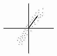
![[PCA Example]](images/rotate.animated.gif)

From Aberystwyth quantitative
biology and analytical biotechnology group
Click on the image above to view how a given set of data can be
made to make sense when viwed from a different direction. Also this denotes
the principal direction along which the data set contains most information.
It is such a direction that we are interested in. As shown in the plot of a typical
data set which again, is concentrated along a particular direction,
we need not spend effort and memory saving the irrelevant parts - once
the principal directions are known using the principal component analysis.
![[Back to Top]](images/icons/first.gif)
![[Previous]](images/icons/prev.gif)
![[Next]](images/icons/next.gif)
![[Last]](images/icons/last.gif)
![[Home]](images/icons/home.gif)
![[Information]](images/icons/info.gif)
PCA Formulation for Shape Classification
Defining the Shape Class Space
A training letter_image can be thought of as a training vector with each
image pixel as the component of that vector. Let X be the Training set
matrix (columns of which are training vectors used
to define shape class) and W be the covariance matrix.
The outer
product of one matrix is product of the matrix with its
transposed form i.e W = X*XT
The L principal components are the first L eigenvectors of the covariance
matrix W arranged in descending order. Since all the elements of the image
are not relevant to represent the image, we choose first L eigen
vectors to represent an image class. Let P be the matrix of the first
L eigenvectors (each eigenvector being a column of P). So, the aim is to calculate
P.
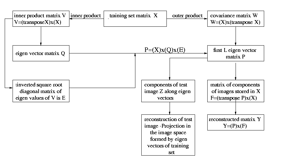
 Figure: Block Diagram showing the steps involved in image
manipulation using PCA to arrive at the eigen vector space of the
training set images and reconstruction of images in this vector space.
To compute W and then P is too time consuming.
Indeed, X is a N by K matrix (where N is the number of elements (pixel) in a
vector (image) and K the number of these training vectors). Hence W is
an N by N matrix. But N is far larger than K.
For example, if 200 images are used, each image having a resolution
of 64 by 64 pixels. K = 200, while N = 64*64 = 4096. Therefore, it is much faster
to compute V, the inner product of X. The inner product of a
matrix is the product of the transposed form of
this matrix by itself. So V is a K by K matrix.It
can be shown that P = X * Q * E where
Q is the eigenvector matrix of V
and E is the inverted square root diagonal matrix of the eigenvalues of V.
The details and proof of this result can be obtained from standard linear algebra books.
Image Reconstruction in the defined space
Let F be the matrix of the components of the faces
stored in the matrix X (the ith column of F forms the composnts of the
ith column of X, which is a face). PCA computes F as follows :
F = PT* X.
Lets Y be the reconstruction matrix from the components
stored in the matrix F. PCA computes Y as
follows : Y = P * F
This method does a great amount of big matrices product, which is a time
consuming operation and the recognition process takes appreciable time depending upon
number of images in the training and recognition sets.
![[Back to Top]](images/icons/first.gif)
![[Previous]](images/icons/prev.gif)
![[Next]](images/icons/next.gif)
![[Last]](images/icons/last.gif)
![[Home]](images/icons/home.gif)
![[Information]](images/icons/info.gif)
Sample Results
Sample results as obtained from Face recognition code are presented here.
Input
The input consists of a training set of grey scale images as shown here.
For each object, the input would be several such images actually
derived from a parent input figure by applying specified vertex and edge perturbations.
Also, the false image training set is given as one having deviations from
the standard image in excess of the specified tolerances.
The number of eigen vectors to compute and the test images are also provided.

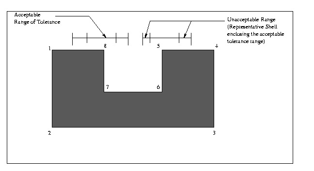
Figure: The shown Polygon was taken up as a case and the
following purturbations were applied to produce the acceptable and non-acceptable
shape class models: Vertices 7 and 8 were given individual perturbations
in the range illustrated for acceptable and non-acceptable ranges. Similarly
vertices 5 and 6 were perturbed in their ranges but simultaneously so as to
keep edge 5-6 vertical.
The actual numerical values and the nature of tolerance definition
may vary and accordingly the enclosing unacceptable range shell too,
but the idea remains that any possible heavy variation in the specified
shape would produce object more similar to those defined by the outer shell
than those in the accepted tolerance range. So these may be accordingly
rejected.
Click on the following animated images to view the complete training set.


Figure: Animated sets for training - Left to right: Desired Tolerances,
Tolerance on left face (inner bound),
Tolerance on left face (upper bound),
Tolerance on right face of hole (lower bound),
Tolerance on right face (upper bound).
The output would be a set of shape classes which shall all be different
in the strict sense of CAD modelling as used today, but each of these would
be identified as the same object from where they originated.
Eigen Vectors

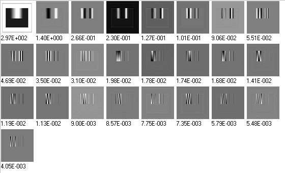
Figure:
These are the EIgen vectors' Reconstruction for the case of training classes taken.
Matching Results
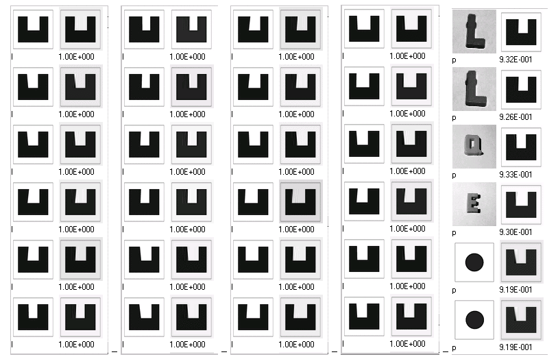
For the Recognition testing, The first 5 images were taken from the admissible
set (l), the remaining being taken 5 each from classes (m),
(n), and (o) while 4 test cases were chosen from (p).
Also, six additional cases were taken which were very dissimilar from the claasses defined.

Figure: The results mapped the corresponding images onto the
parent classes,
i.e. while trying to match with the standard class - l,
it gave wrong recognition. In cases of entirely different images, the weighted eigen vectors
are smaller and can be threshholded*.
Failure case: The first image, though actually belonging to the standard class, was rejected
and mapped to be belonging to class (o) and it is very difficult to threshold such
a failure case since the weighted eigen values are close to the standard value.
*The threshhold value works definitively
only with closely resembling objects. A simple approach to thresholding on the basis of
the projection of test object onto the eigen space createdd, i.e. the weighted
eigen values, does not necessarily yield conclusive results. An entirely different object might
map onto the eigen space well enough to produce a resultant magnitude of weighted eigen values
in the range produced by admissable objects.
![[Back to Top]](images/icons/first.gif)
![[Previous]](images/icons/prev.gif)
![[Next]](images/icons/next.gif)
![[Last]](images/icons/last.gif)
![[Home]](images/icons/home.gif)
![[Information]](images/icons/info.gif)
Limitations
- As pointed out before, a major drawback of the algorithm is that it
is not robust with reference to strange objects i.e. ones for which it has not been
trained before. Given a set of classes and a fresh input image, the algorithm
computes the minimum distance of the image in projected space, from each of the classes
and classifies it into the one for which the distance is minimum.
- The current training class generation code is limited to standard identified
objects. The purturbations and tolerances also have to be defined discretely
for data vectors' generation. Though, extension of this is fairly trivial and
mundane, the current code does not facilitate this. Such an extension may be
made simply by defining more shape categories and allowing the user freedom
of choice. Yet, for the cases undertaken, the code is crisp, making use of standard
Imagemagick library,
executing in batch mode to generate several hundreds of images as desired.
- The standard code obtained from the
Face recognition group, could not be recompiled to tailor it to the needs of
the current study. Instead, attempt to construct fresh code for PCA using the
same algorithm, in Python is underway.
The code successfully does the eigen value calculations from imported images, yet the
output format for images (exporting the output values) is to be developed.
Conclusions
The return value of weighted eigenvectors do not seem to bear a definite
trend for objects which are widely different from those of the training classes.
It is difficult to say at this stage whether these values can be threshholded
successfully to categorically reject an entirely new image, for which
the program has not been trained beforehand. But nevertheless, the algorithm
works remarkably well for objects close to those present in the training set.
As seen in the results presented in the case studies done in this work,
it is capable of classifying closely similar objects with fairly high accuracy.
Given the nature of the problem at hand, i.e. Tolerance definition and identification,
this property is particularly useful. Moreover, it is only unlikely in a manufacturing
process that a strange object is encounterd from a standard machined output.
This process, though tested largely for artificially generated images, works smoothly
with real-life photographs as well, with similar characteristics. The tool may therefore
be very suitably applied to a manufacturing process where it is required to detect
faults in objects through various tolerance definitions.
![[Back to Top]](images/icons/first.gif)
![[Previous]](images/icons/prev.gif)
![[Next]](images/icons/next.gif)
![[Last]](images/icons/last.gif)
![[Home]](images/icons/home.gif)
![[Information]](images/icons/info.gif)
References
- Goswami,A. Identification of Partially visible Shape Classes, July 1999
Indian Institute of Technology, Kanpur, Dept of mechanical engg.
- Ziyad N.A. &
GilmoreE.T. & TuggleK. & ChouikhaM.F., Howard University, Department of Electrical Engineering, Washington
,Image Representation Recovery and analysis using Principal Component Analysis
- Two
Dimensional Image Processing
-
Srinivas Akella's Research
- Face Recognition Group Home Page
- PCA Revisited
- Related Links
![[Back to Top]](images/icons/first.gif)
![[Previous]](images/icons/prev.gif)
![[Next]](images/icons/next.gif)
![[Last]](images/icons/last.gif)
![[Home]](images/icons/home.gif)
![[Information]](images/icons/info.gif)
This report was prepared by Gagan Deep Arora and Ravi P.Srivastava as a part
of the project component in the
Course on Computer Aided Engineering Design
in the July-December Semester, 1999.
(Instructor :
Amitabha Mukerjee )
[CAED COURSE LECTURES HOME PAGE]
![[PCA Example]](images/rotate.animated.gif)
